Developer manual#
Developer tips#
Compiling Hermes-3 quickly#
After compiling Hermes-3 and changing something, you can avoid unnecessary recompilation of unchanged files. Simply enter the build directory and do:
make -j 4
Where 4 will make it compile using 4 cores. You can increase or decrease this as necessary.
Sometimes, CMake will think that it needs to recompile parts of BOUT++ even if it wasn’t changed.
To stop this try adding the flag -DHERMES_UPDATE_GIT_SUBMODULE=OFF in your CMake command.
This and other useful options can be found in hermes-3/CMakeLists.txt.
Compiling documentation#
The Hermes-3 documentation is built using Sphinx and Doxygen. It’s written in ReStructuredText (RST), which is a markup language similar to Markdown. Doxygen generates automatic documentation based on the C++ code, while Sphinx handles everything else.
Editing documentation is much easier if you can compile it locally using the following steps:
Install Sphinx and our theme in your Python environment:
pip install sphinx sphinx_book_theme
Install Doxygen (modify as necessary for your OS) and Breathe, the package that connects it to Sphinx:
sudo apt install doxygen
Install Breathe (modify as necessary for your OS):
pip install breathe
Run Doxygen - this will parse the C++ code:
cd hermes-3/docs/doxygen
Doxygen doxyfile
Run Sphinx - this will parse the RST files and generate the documentation.
sphinxandbuildare the source and build directories, respectively.cd hermes-3/docs sphinx-build sphinx build
Open the generated HTML files, either by double clicking on the file in your browser, or some other way. If you use VS Code locally or on a remote machine through SSH, you can use the extension Live Preview which can stream it to your browser.
Debugging: running for one iteration#
Any BOUT++ code can be run for just one right-hand side (RHS) iteration. This will run instantly for any simulation and not need any kind of solver convergence, making it ideal for debugging.
This can be done by setting the following in the input file:
nout = 0
The timestep setting will be ignored.
Debugging: printing values#
When debugging, it can be useful to print things out. This is simple in C++.
For example, if you want to print the value of the variable particle_flow, do:
output << "\n*******************************\n"
output << "particle_flow: " << particle_flow << "\n"
output << "*******************************\n"
Which will result in:
*******************************
particle_flow: 0.123456
*******************************
Sometimes you need to deal with printing whole fields. In this case, it is useful
to print out every cell value along with its coordinates. The below code snippet will
do this for the variable Tn:
or(int ix=0; ix < mesh->LocalNx ; ix++){
   for(int iy=0; iy < mesh->LocalNy ; iy++){
       for(int iz=0; iz < mesh->LocalNz; iz++){

         std::string string_count = std::string("(") + std::to_string(ix) + std::string(",") + std::to_string(iy)+ std::string(",") + std::to_string(iz) + std::string(")");
         output << string_count + std::string(": ") + std::to_string(Tn(ix,iy,iz)) + std::string("; ");
       }
   }
 output << "\n";
 }
The output will look something like:
(0,0,0): 0.123456; (0,0,1): 0.654321; (0,0,2): 0.987654; (0,1,0): 0.123456; (0,1,1): 0.654321; (0,1,2): 0.987654;
(1,0,0): 0.123456; (1,0,1): 0.654321; (1,0,2): 0.987654; (1,1,0): 0.123456; (1,1,1): 0.654321; (1,1,2): 0.987654;
...
Note that there are multiple ways to print out values in C++, and both std::string(text) and "text" are valid.
Debugging: segmentation faults#
Segmentation faults can be frustrating because they give very little verbosity. In practice, the most common cause is trying to access a variable that hasn’t been initialised yet. The easiest way to debug this is to carefully review the new lines of code to make sure all variables exist and have been declared and initialised. If this is tricky, another simple way is to comment out large parts of the code until the segmentation fault disappears, helping to narrow down its location.
While the above methods are very simple and can be effective, debugging tools such as gdb or valgrind can be used to find the segmentation fault as well.
Debugging: compiling in debug mode#
This can be a useful way to catch errors. Please see the relevant page in the BOUT++ documentation.
Header vs. implementation files#
C++ allows you to split code into implementation (.cxx) and header (.hxx) files.
The convention of what should be in each one is not consistent in Hermes-3 at
the moment. The most common standard is for the header file to contain all of the
variable and class declarations and the implementation file to contain the rest.
An example of this is in the evolve_density component - see the
implementation file
and the header file.
Data types#
Hermes-3 casts its variables in a variety of BOUT++ classes. Floats are
usually represented as BoutReal, and fields as Field3D. Note that
Hermes-3 always runs “in 3D” - when configured in 1D, the x and z dimensions
are of unit length. See relevant BOUT++ docs
for more info. There is also a data type called Options which is equivalent
to a Python dictionary with extra functionality, and is used to store input
options, the entire simulation state and many other data.
Adding new settings#
This is simple and uses the following syntax:
bndry_flux = options["bndry_flux"]
                  .doc("Allow flows through radial boundaries")
                  .withDefault<bool>(true);
The variable must also be declared in the corresponding header file.
Adding new diagnostics#
Adding new diagnostics is also simple, provided there is already an outputVars
function set up in your component. This is usually located at the end of the
implementation file. See this example from evolve_momentum.cxx:
void EvolveMomentum::outputVars(Options &state) {
AUTO_TRACE();
// Normalisations
auto Nnorm = get<BoutReal>(state["Nnorm"]);
auto Omega_ci = get<BoutReal>(state["Omega_ci"]);
auto Cs0 = get<BoutReal>(state["Cs0"]);

state[std::string("NV") + name].setAttributes(
      {{"time_dimension", "t"},
      {"units", "kg / m^2 / s"},
      {"conversion", SI::Mp * Nnorm * Cs0},
      {"standard_name", "momentum"},
      {"long_name", name + " parallel momentum"},
      {"species", name},
      {"source", "evolve_momentum"}});
Each diagnostic is saved with metadata, which is available in xHermes, e.g.
ds["Nd"].attrs()
- time_dimension
This indicates that the variable is time evolving. If you remove this line, it will be saved only at the first RHS evaluation.
- units
A string showing the units for post-processing. xHermes picks this up.
- conversion
A float representing the normalisation factor. xHermes picks this up to do automatic conversion to SI units.
- standard_name, long_name
We aren’t consistent on what should be in each, but they are meant to describe the variables in post-processing.
- species, source
The relevant species and component that the diagnostic is coming from
What is “Options”?#
Options is a dictionary-like class originally developed for parsing BOUT++ options. In Hermes-3, it is used as a general purpose dictionary.
Getting/setting values#
Hermes-3 has a system to prevent quantities from being modified after they are used.
This is important as it uses a single dictionary-like state class to hold all of
the variables in one place, which could allow some components to overwrite others.
In component.hxx there is the function get, which once called sets the
“final” and “final-domain” attributes:
When you call set, these attributes are checked for, so that if they have
already been “gotten”, they can’t be set again:
Options& set(Options& option, T value) {
// Check that the value has not already been used
#if CHECKLEVEL >= 1
if (option.hasAttribute("final")) {
   throw BoutException("Setting value of {} but it has already been used in {}.",
                        option.name(), option.attributes["final"].as<std::string>());
}
if (option.hasAttribute("final-domain")) {
   throw BoutException("Setting value of {} but it has already been used in {}.",
                        option.name(),
                        option.attributes["final-domain"].as<std::string>());
}

if (hermesDataInvalid(value)) {
   throw BoutException("Setting invalid value for '{}'", option.str());
}
#endif
There is a special use case which allows you to use this “locking” scheme for only
the domain cells, leaving the guard cells to be settable using getNoBoundary:
T getNoBoundary(const Options& option, const std::string& location = "") {
#if CHECKLEVEL >= 1
// Mark option as final inside the domain
const_cast<Options&>(option).attributes["final-domain"] = location;
#endif
return getNonFinal<T>(option);
}
And there is a corresponding setBoundary that can be used for BC operations:
Options& setBoundary(Options& option, T value) {
// Check that the value has not already been used
#if CHECKLEVEL >= 1
if (option.hasAttribute("final")) {
   throw BoutException("Setting boundary of {} but it has already been used in {}.",
                        option.name(), option.attributes["final"].as<std::string>());
}
#endif
option.force(std::move(value));
return option;
}
These functions take a second argument which tells you where they were set, which is easier for debugging.
They are wrapped into additional functions, GET_VALUE and GET_NOBOUNDARY which automatically
include this argument.
Please review component.hxx for more details.
Looping over cells#
BOUT++ provides a really easy way to loop over the domain using BOUT_FOR and
similar loops, see BOUT++ docs.
There is a way to way to tell if you are in the core or not. The mesh object
has a function to indicate if the coordinate is in a periodic region or not.
Only the core is periodic. See below for an example from evolve_pressure.cxx
which makes sure a pressure source is set to zero outside of the core:
if (p_options["source_only_in_core"]
   .doc("Zero the source outside the closed field-line region?")
   .withDefault<bool>(false)) {
 for (int x = mesh->xstart; x <= mesh->xend; x++) {
   if (!mesh->periodicY(x)) {
     // Not periodic, so not in core
     for (int y = mesh->ystart; y <= mesh->yend; y++) {
       for (int z = mesh->zstart; z <= mesh->zend; z++) {
         source(x, y, z) = 0.0;
       }
     }
   }
 }
Code structure#
A hermes-3 model, like all BOUT++ models,
is an implementation of a set of Ordinary Differential Equations
(ODEs). The time integration solver drives the simulation, calling the
Hermes::rhs function to calculate the time-derivatives of all the
evolving variables.
The calculation of the time derivatives is coordinated by passing a state object between components. The state is a nested tree, and can have values inserted and retrieved by the components. The components are created and then run by a scheduler, based on settings in the input (BOUT.inp) file.
For example a transport simulation with deuterium and tritium ions and atoms has an input file specifying the components
[hermes]
components = d+, d, t+, t, e, collisions, sheath_boundary, recycling, reactions
The governing equations for each species are specified e.g.
[d+]
type = evolve_density, evolve_momentum, evolve_pressure, anomalous_diffusion
AA = 2   # Atomic mass
charge = 1
and other components have their configuration options e.g. for reactions:
[reactions]
type = (
        d + e -> d+ + 2e,   # Deuterium ionisation
        t + e -> t+ + 2e,   # Tritium ionisation
       )
In terms of design patterns, the method used here is essentially a combination of the Encapsulate Context and Command patterns.
Simulation state#
The simulation state is passed between components, and is a tree of objects (Options objects). At the start of each iteration (rhs call) a new state is created and contains:
timeBoutReal, the current simulation timelinearbool. True if the time integrator expects a linear response.unitssecondsMultiply by this to get units of secondseVTemperature normalisationTeslaMagnetic field normalisationmetersLength normalisationinv_meters_cubedDensity normalisation
so the temperature normalisation can be extracted using:
BoutReal Tnorm = state["units"]["eV"];
As the components of a model are run, they set, modify and use values stored in this state. To ensure that components use consistent names for their input and output variables, a set of conventions are used for new variables which are added to the state:
speciesPlasma specieseElectron speciesspecies1Example “h”, “he+2”AAAtomic mass, proton = 1chargeCharge, in units of proton charge (i.e. electron=-1)densitymomentumParallel momentumpressurevelocityParallel velocitytemperaturecollision_frequencyNormalised collision frequencydensity_sourceNormalised particle sourcemomentum_sourceNormalised momentum sourceenergy_sourceNormalised energy sourceparticle_flow_xlowNormalised particle flow through lower X cell faceparticle_flow_ylowNormalised particle flow through lower Y cell facemomentum_flow_xlowNormalised momentum flow through lower X cell facemomentum_flow_ylowNormalised momentum flow through lower Y cell faceenergy_flow_xlowNormalised energy flow through lower X cell faceenergy_flow_ylowNormalised energy flow through lower Y cell face
fieldsvorticityphiElectrostatic potentialAparElectromagnetic potential b dot A in induction termsApar_flutterThe electromagnetic potential (b dot A) in flutter termsDivJdiaDivergence of diamagnetic currentDivJcolDivergence of collisional currentDivJextraDivergence of current, including 2D parallel currentclosures. Not including diamagnetic, parallel current due to flows, or polarisation currents
For example to get the electron density:
Field3D ne = state["species"]["e"]["density"];
This way of extracting values from the state will print the value to
the log file, and is intended mainly for initialisation. In
Component::transform() and Component::finally() functions which run
frequently, faster access methods are used which don’t print to the
log. To get a value:
Field3D ne = get<Field3D>(state["species"]["e"]["density"]);
If the value isn’t set, or can’t be converted to the given type,
then a BoutException will be thrown.
To set a value in the state, there is the set() function:
set(state["species"]["h"]["density"], ne);
A common need is to add or subtract values from fields, such as density sources:
add(state["species"]["h"]["density_source"], recombination_rate);
subtract(state["species"]["h+"]["density_source"], recombination_rate);
Notes:
When checking if a subsection exists, use
option.isSection, sinceoption.isSetis false if it is a section and not a value.The species name convention is that the charge state is last, after the
+or-sign:n2+is a singly charged nitrogen molecule, whilen+2is a +2 charged nitrogen atom.
Components#
The basic building block of all Hermes-3 models is the
Component. This defines an interface to a class which takes a state
(a tree of dictionaries/maps), and transforms (modifies) it. After
all components have modified the state in turn, all components may
then implement a finally method to take the final state but not
modify it. This allows two components to depend on each other, but
makes debugging and testing easier by limiting the places where the
state can be modified.
-
struct Component
Interface for a component of a simulation model
The constructor of derived types should have signature (std::string name, Options &options, Solver *solver)
Subclassed by AnomalousDiffusion, BinormalSTPM, ClassicalDiffusion, Collisions, DetachmentController, DiamagneticDrift, Electromagnetic, ElectronForceBalance, ElectronViscosity, EvolveDensity, EvolveEnergy, EvolveMomentum, EvolvePressure, FixedDensity, FixedFractionIons, FixedFractionRadiation< CoolingCurve >, FixedTemperature, FixedVelocity, IonViscosity, Ionisation, Isothermal, NeutralBoundary, NeutralFullVelocity, NeutralMixed, NeutralParallelDiffusion, NoFlowBoundary, PolarisationDrift, Quasineutral, ReactionBase, Recycling, RelaxPotential, SNBConduction, SOLKITNeutralParallelDiffusion, ScaleTimeDerivs, SetTemperature, SheathBoundary, SheathBoundaryInsulating, SheathBoundarySimple, SheathClosure, SimpleConduction, SimplePump, SoundSpeed, TemperatureFeedback, ThermalForce, Transform, UpstreamDensityFeedback, Vorticity, ZeroCurrent
Public Functions
-
virtual void transform(Options &state) = 0
Modify the given simulation state All components must implement this function
-
inline virtual void finally(const Options &state)
Use the final simulation state to update internal state (e.g. time derivatives)
-
inline virtual void outputVars(Options &state)
Add extra fields for output, or set attributes e.g docstrings.
-
inline virtual void restartVars(Options &state)
Add extra fields to restart files.
-
inline virtual void precon(const Options &state, BoutReal gamma)
Preconditioning.
Public Static Functions
-
static std::unique_ptr<Component> create(const std::string &type, const std::string &name, Options &options, Solver *solver)
Create a Component
- Parameters:
type – The name of the component type to create (e.g. “evolve_density”)
name – The species/name for this instance.
options – Component settings: options[name] are specific to this component
solver – Time-integration solver
-
virtual void transform(Options &state) = 0
Components are usually defined in separate files; sometimes multiple components in one file if they are small and related to each other (e.g. atomic rates for the same species). To be able to create components, they need to be registered in the factory. This is done in the header file using a code like:
#include "component.hxx"

struct MyComponent : public Component {
  MyComponent(const std::string &name, Options &options, Solver *solver);
  ...
};

namespace {
RegisterComponent<MyComponent> registercomponentmine("mycomponent");
}
where MyComponent is the component class, and “mycomponent” is the
name that can be used in the BOUT.inp settings file to create a
component of this type. Note that the name can be any string except it
can’t contain commas or brackets (), and shouldn’t start or end with
whitespace.
Inputs to the component constructors are:
namealloptionssolver
The name is a string labelling the instance. The alloptions tree contains at least:
alloptions[name]options for this instancealloptions['units']
Component scheduler#
The simulation model is created in Hermes::init by a call to the ComponentScheduler:
scheduler = ComponentScheduler::create(options, Options::root(), solver);
and then in Hermes::rhs the components are run by a call:
scheduler->transform(state);
The call to ComponentScheduler::create() treats the “components”
option as a comma-separated list of names. The order of the components
is the order that they are run in. For each name in the list, the
scheduler looks up the options under the section of that name.
[hermes]
components = component1, component2

[component1]

# options to control component1

[component2]

# options to control component2
This would create two Component objects, of type component1 and
component2. Each time Hermes::rhs is run, the transform
functions of component1 amd then component2 will be called,
followed by their finally functions.
It is often useful to group components together, for example to
define the governing equations for different species. A type setting
in the option section overrides the name of the section, and can be another list
of components
[hermes]
components = group1, component3

[group1]
type = component1, component2

# options to control component1 and component2

[component3]

# options to control component3
This will create three components, which will be run in the order
component1, component2, component3: First all the components
in group1, and then component3.
-
class ComponentScheduler
Creates and schedules model components
Currently only one implementation, but in future alternative scheduler types could be created. There is therefore a static create function which in future could switch between types.
Public Functions
-
void transform(Options &state)
Run the scheduler, modifying the state. This calls all components’ transform() methods, then all component’s finally() methods.
-
void outputVars(Options &state)
Add metadata, extra outputs. This would typically be called only for writing to disk, rather than every internal timestep.
-
void restartVars(Options &state)
Add variables to restart files.
-
void precon(const Options &state, BoutReal gamma)
Preconditioning.
Public Static Functions
-
static std::unique_ptr<ComponentScheduler> create(Options &scheduler_options, Options &component_options, Solver *solver)
Inputs
- Parameters:
scheduler_options – Configuration of the scheduler Should contain “components”, a comma-separated list of component names
component_options – Configuration of the components.
<name>
type = Component classes, … If not provided, the type is the same as the name Multiple classes can be given, separated by commas. All classes will use the same Options section.
… Options to control the component(s)
solver – Used for time-dependent components to evolve quantities
-
void transform(Options &state)
Tests#
The specification of the Toro tests used here is taken from Walker (2012), originally from Toro’s book Riemann Solvers and Numerical Methods for Fluid Dynamics.
1D fluid (MMS)#
tests/integrated/1D-fluid
This convergence test using the Method of Manufactured Solutions (MMS) solves fluid equations in the pressure form:

Sod shock#
tests/integrated/sod-shock and tests/integrated/sod-shock-energy
Euler equations in 1D. Starting from a state with a jump at the middle of the domain. Left state density, velocity and pressure are \(\left(\rho_L, u_L, p_L\right) = \left(1.0, 0, 1.0\right)\) Right state \(\left(\rho_R, u_R, p_R\right) = \left(0.125, 0, 0.1\right)\). The result is shown in figure below at time \(t = 0.2\) for different resolutions in a domain of length 1. The solid black line is the analytic solution.
When evolving pressure the position of the shock front lags the analytic solution, with the pressure behind the front slightly too high. This is a known consequence of solving the Euler equations in non-conservative form. If instead we evolve energy (internal + kinetic) then the result is much closer to the analytic solution.
Toro test 1#
tests/integrated/toro-1
Toro’s test problem #1, from Riemann Solvers and Numerical Methods for Fluid Dynamics is a variation of Sod’s shock tube problem. The left state is moving into the right, increasing the speed of the resulting shock. Left state \(\left(\rho_L, u_L, p_L\right) = \left(1.0, 0.75, 1.0\right)\) Right state \(\left(\rho_R, u_R, p_R\right) = \left(0.125, 0, 0.1\right)\). The size of the domain is 5, and the reference result is given at time \(t = 0.8\).
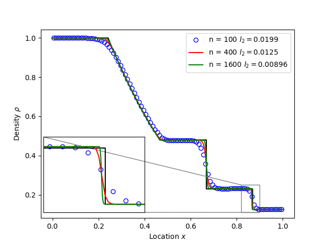
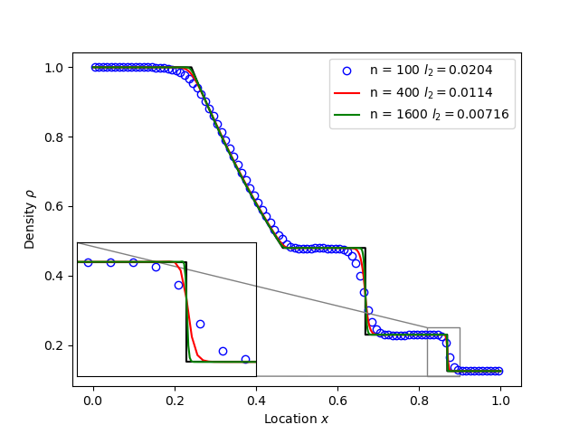
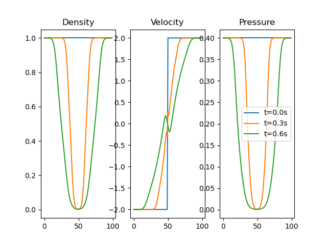
Toro test 2#
tests/integrated/toro-2 and tests/integrated/toro-2-energy
Toro’s test problem #2 tests robustness to diverging flows and near-zero densities. The initial state has constant density and temperature, but a jump in velocity. Left state \(\left(\rho_L, u_L, p_L\right) = \left(1.0, -2.0, 0.4\right)\) Right state \(\left(\rho_R, u_R, p_R\right) = \left(1.0, 2.0, 0.4\right)\). The result in a domain of length 5 at time \(t=0.6\) is shown below.
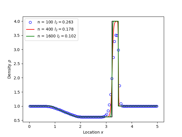
Toro test 3#
tests/integrated/toro-3 and tests/integrated/toro-3-energy
Toro’s test problem #3 contains a strong shock close to a contact discontinuity. Left initial state \(\left(\rho_L, u_L, p_L\right) = \left(1.0, 0, 1000.0\right)\) Right state \(\left(\rho_R, u_R, p_R\right) = \left(1.0, 0, 0.01\right)\). Time \(t = 0.04\).
When evolving pressure, the simulation is robust but the density peak does not converge to the analytic solution (solid black line):

However by evolving energy the result converges towards the analytic solution:
Toro test 4#
tests/integrated/toro-4 and tests/integrated/toro-4-energy
Toro’s test problem #4 produces two right-going shocks with a contact between them. Left state \(\left(\rho_L, u_L, p_L\right) = \left(5.99924, 19.5975, 460.894\right)\) Right state \(\left(\rho_R, u_R, p_R\right) = \left(5.99242, -6.19633, 46.0950\right)\). Result at time \(t = 0.15\).
Toro test 5#
tests/integrated/toro-5 and tests/integrated/toro-5-energy
The initial conditions for Toro’s test problem #5 are the same as test #3, but the whole system is moving to the left at a uniform speed. The velocity is chosen so that the contact discontinuity remains almost stationary at the initial jump location. Left state \(\left(\rho_L, u_L, p_L\right) = \left(1, -19.59745, 1000.0\right)\) Right state \(\left(\rho_R, u_R, p_R\right) = \left(1, -19.59745, 0.01\right)\). Result at time \(t = 0.03\).
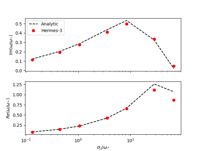
Drift wave#
tests/integrated/drift-wave
This calculates the growth rate and frequency of a resistive drift wave with finite electron mass.
The equations solved are:
Linearising around a stationary background with constant density \(n_0\) and temperature \(T_0\), using \(\frac{\partial}{\partial t}\rightarrow -i\omega\) gives:
where the radial density length scale coming from the radial \(E\times B\) advection of density is defined as
Substituting and rearranging gives:
or
where
This is a cubic dispersion relation, so we find the three roots (using NumPy), and choose the root with the most positive growth rate (imaginary component of \(\omega\)).
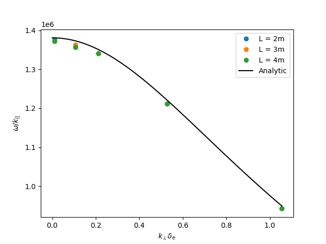
Alfven wave#
The equations solved are
Linearising around a stationary background with constant density \(n_0\) and temperature \(T_0\), using \(\frac{\partial}{\partial t}\rightarrow -i\omega\) gives:
Rearranging results in a quadratic dispersion relation:
where \(V_A = B / \sqrt{\mu_0 n_0 m_i}\) is the Alfven speed, and \(c / \omega_{pe} = \sqrt{m_e / \left(\mu_0 n_0 e^2\right)}\) is the electron skin depth.
When collisions are neglected, we obtain the result
Collision frequency selection#
There are two simple integrated tests to make sure that the collision frequency selection is correct
across neutral_mixed, evolve_pressure, ion_viscosity and neutral_parallel_diffusion.
A minimal 3D geometry is run for one RHS evaluation, and the test checks the log file
to make sure the correct collisionalities were selected. One of the tests is for the multispecies
mode across all components, while the other is for braginskii for plasma and afn for neutrals.