Developer manual#
Developer tips#
Compiling Hermes-3 quickly#
After compiling Hermes-3 and changing something, you can avoid unnecessary recompilation of unchanged files. Simply enter the build directory and do:
make -j 4
Where 4 will make it compile using 4 cores. You can increase or decrease this as necessary.
Sometimes, CMake will think that it needs to recompile parts of BOUT++ even if it wasn’t changed.
To stop this try adding the flag -DHERMES_UPDATE_GIT_SUBMODULE=OFF in your CMake command.
This and other useful options can be found in hermes-3/CMakeLists.txt.
Compiling documentation#
The Hermes-3 documentation is built using Sphinx and Doxygen. It’s written in ReStructuredText (RST), which is a markup language similar to Markdown. Doxygen generates automatic documentation based on the C++ code, while Sphinx handles everything else.
Editing documentation is much easier if you can compile it locally using the following steps:
Install Sphinx and our theme in your Python environment:
pip install sphinx sphinx_book_theme
Install Doxygen (modify as necessary for your OS) and Breathe, the package that connects it to Sphinx:
sudo apt install doxygen
Install Breathe (modify as necessary for your OS):
pip install breathe
Run Doxygen - this will parse the C++ code:
cd hermes-3/docs/doxygen
doxygen Doxyfile
Run Sphinx - this will parse the RST files and generate the documentation.
sphinxandbuildare the source and build directories, respectively.cd hermes-3/docs sphinx-build sphinx build
Open the generated HTML files, either by double clicking on the file in your browser, or some other way. If you use VS Code locally or on a remote machine through SSH, you can use the extension Live Preview which can stream it to your browser.
Debugging: running for one iteration#
Any BOUT++ code can be run for just one right-hand side (RHS) iteration. This will run instantly for any simulation and not need any kind of solver convergence, making it ideal for debugging.
This can be done by setting the following in the input file:
nout = 0
The timestep setting will be ignored.
Debugging: printing values#
When debugging, it can be useful to print things out. This is simple in C++.
For example, if you want to print the value of the variable particle_flow, do:
output << "\n*******************************\n"
output << "particle_flow: " << particle_flow << "\n"
output << "*******************************\n"
Which will result in:
*******************************
particle_flow: 0.123456
*******************************
Sometimes you need to deal with printing whole fields. In this case, it is useful
to print out every cell value along with its coordinates. The below code snippet will
do this for the variable Tn:
or(int ix=0; ix < mesh->LocalNx ; ix++){
   for(int iy=0; iy < mesh->LocalNy ; iy++){
       for(int iz=0; iz < mesh->LocalNz; iz++){

         std::string string_count = std::string("(") + std::to_string(ix) + std::string(",") + std::to_string(iy)+ std::string(",") + std::to_string(iz) + std::string(")");
         output << string_count + std::string(": ") + std::to_string(Tn(ix,iy,iz)) + std::string("; ");
       }
   }
 output << "\n";
 }
The output will look something like:
(0,0,0): 0.123456; (0,0,1): 0.654321; (0,0,2): 0.987654; (0,1,0): 0.123456; (0,1,1): 0.654321; (0,1,2): 0.987654;
(1,0,0): 0.123456; (1,0,1): 0.654321; (1,0,2): 0.987654; (1,1,0): 0.123456; (1,1,1): 0.654321; (1,1,2): 0.987654;
...
Note that there are multiple ways to print out values in C++, and both std::string(text) and "text" are valid.
Debugging: segmentation faults#
Segmentation faults can be frustrating because they give very little verbosity. In practice, the most common cause is trying to access a variable that hasn’t been initialised yet. The easiest way to debug this is to carefully review the new lines of code to make sure all variables exist and have been declared and initialised. If this is tricky, another simple way is to comment out large parts of the code until the segmentation fault disappears, helping to narrow down its location.
While the above methods are very simple and can be effective, debugging tools such as gdb or valgrind can be used to find the segmentation fault as well.
Debugging: compiling in debug mode#
This can be a useful way to catch errors. Please see the relevant page in the BOUT++ documentation.
Header vs. implementation files#
C++ allows you to split code into implementation (.cxx) and header (.hxx) files.
The convention of what should be in each one is not consistent in Hermes-3 at
the moment. The most common standard is for the header file to contain all of the
variable and class declarations and the implementation file to contain the rest.
An example of this is in the evolve_density component - see the
implementation file
and the header file.
Data types#
Hermes-3 casts its variables in a variety of BOUT++ classes. Floats are
usually represented as BoutReal, and fields as Field3D. Note that
Hermes-3 always runs “in 3D” - when configured in 1D, the x and z dimensions
are of unit length. See relevant BOUT++ docs
for more info. There is also a data type called Options which is equivalent
to a Python dictionary with extra functionality, and is used to store input
options, the entire simulation state and many other data. Finally,
there is the GuardedOptions datatype, which wraps an Options
object and controls access to its contents.
Adding new settings#
This is simple and uses the following syntax:
bndry_flux = options["bndry_flux"]
                  .doc("Allow flows through radial boundaries")
                  .withDefault<bool>(true);
The variable must also be declared in the corresponding header file.
Adding new diagnostics#
Adding new diagnostics is also simple, provided there is already an outputVars
function set up in your component. This is usually located at the end of the
implementation file. See this example from evolve_momentum.cxx:
void EvolveMomentum::outputVars(Options &state) {
AUTO_TRACE();
// Normalisations
auto Nnorm = get<BoutReal>(state["Nnorm"]);
auto Omega_ci = get<BoutReal>(state["Omega_ci"]);
auto Cs0 = get<BoutReal>(state["Cs0"]);

state[std::string("NV") + name].setAttributes(
      {{"time_dimension", "t"},
      {"units", "kg / m^2 / s"},
      {"conversion", SI::Mp * Nnorm * Cs0},
      {"standard_name", "momentum"},
      {"long_name", name + " parallel momentum"},
      {"species", name},
      {"source", "evolve_momentum"}});
Each diagnostic is saved with metadata, which is available in xHermes, e.g.
ds["Nd"].attrs()
- time_dimension
This indicates that the variable is time evolving. If you remove this line, it will be saved only at the first RHS evaluation.
- units
A string showing the units for post-processing. xHermes picks this up.
- conversion
A float representing the normalisation factor. xHermes picks this up to do automatic conversion to SI units.
- standard_name, long_name
We aren’t consistent on what should be in each, but they are meant to describe the variables in post-processing.
- species, source
The relevant species and component that the diagnostic is coming from
What is “Options”?#
Options is a dictionary-like class originally developed for parsing BOUT++ options. In Hermes-3, it is used as a general purpose dictionary.
Getting/setting values#
Hermes-3 has a system to prevent quantities from being modified after they are used.
This is important as it uses a single dictionary-like state class to hold all of
the variables in one place, which could allow some components to overwrite others.
In component.hxx there is the function get, which once called sets the
“final” and “final-domain” attributes:
T get(const Options& option, const std::string& location = "") {
#if CHECKLEVEL >= 1
// Mark option as final, both inside the domain and the boundary
const_cast<Options&>(option).attributes["final"] = location;
const_cast<Options&>(option).attributes["final-domain"] = location;
#endif
return getNonFinal<T>(option);
}
When you call set, these attributes are checked for, so that if they have
already been “gotten”, they can’t be set again:
Options& set(Options& option, T value) {
// Check that the value has not already been used
#if CHECKLEVEL >= 1
if (option.hasAttribute("final")) {
   throw BoutException("Setting value of {} but it has already been used in {}.",
                        option.name(), option.attributes["final"].as<std::string>());
}
if (option.hasAttribute("final-domain")) {
   throw BoutException("Setting value of {} but it has already been used in {}.",
                        option.name(),
                        option.attributes["final-domain"].as<std::string>());
}

if (hermesDataInvalid(value)) {
   throw BoutException("Setting invalid value for '{}'", option.str());
}
#endif
There is a special use case which allows you to use this “locking” scheme for only
the domain cells, leaving the guard cells to be settable using getNoBoundary:
T getNoBoundary(const Options& option, const std::string& location = "") {
#if CHECKLEVEL >= 1
// Mark option as final inside the domain
const_cast<Options&>(option).attributes["final-domain"] = location;
#endif
return getNonFinal<T>(option);
}
And there is a corresponding setBoundary that can be used for BC operations:
Options& setBoundary(Options& option, T value) {
// Check that the value has not already been used
#if CHECKLEVEL >= 1
if (option.hasAttribute("final")) {
   throw BoutException("Setting boundary of {} but it has already been used in {}.",
                        option.name(), option.attributes["final"].as<std::string>());
}
#endif
option.force(std::move(value));
return option;
}
All of these functions are overloaded to accept both Options and
GuardedOptions objects.
These functions take a second argument which tells you where they were set, which is easier for debugging.
They are wrapped into additional functions, GET_VALUE and GET_NOBOUNDARY which automatically
include this argument.
Please review component.hxx for more details.
Looping over cells#
BOUT++ provides a really easy way to loop over the domain using BOUT_FOR and
similar loops, see BOUT++ docs.
There is a way to way to tell if you are in the core or not. The mesh object
has a function to indicate if the coordinate is in a periodic region or not.
Only the core is periodic. See below for an example from evolve_pressure.cxx
which makes sure a pressure source is set to zero outside of the core:
if (p_options["source_only_in_core"]
   .doc("Zero the source outside the closed field-line region?")
   .withDefault<bool>(false)) {
 for (int x = mesh->xstart; x <= mesh->xend; x++) {
   if (!mesh->periodicY(x)) {
     // Not periodic, so not in core
     for (int y = mesh->ystart; y <= mesh->yend; y++) {
       for (int z = mesh->zstart; z <= mesh->zend; z++) {
         source(x, y, z) = 0.0;
       }
     }
   }
 }
Code structure#
A hermes-3 model, like all BOUT++ models,
is an implementation of a set of Ordinary Differential Equations
(ODEs). The time integration solver drives the simulation, calling the
Hermes::rhs function to calculate the time-derivatives of all the
evolving variables.
The calculation of the time derivatives is coordinated by passing a state object between components. The state is a nested tree, and can have values inserted and retrieved by the components. The components are created and then run by a scheduler, based on settings in the input (BOUT.inp) file.
For example a transport simulation with deuterium and tritium ions and atoms has an input file specifying the components
[hermes]
components = (d+, d, t+, t, e, braginskii_collisions,
              braginskii_friction, braginskii_heat_exchange,
              sheath_boundary, recycling, reactions,
              braginskii_conduction)
The governing equations for each species are specified e.g.
[d+]
type = evolve_density, evolve_momentum, evolve_pressure, anomalous_diffusion
AA = 2   # Atomic mass
charge = 1
and other components have their configuration options e.g. for reactions:
[reactions]
type = (
        d + e -> d+ + 2e,   # Deuterium ionisation
        t + e -> t+ + 2e,   # Tritium ionisation
       )
In terms of design patterns, the method used here is essentially a combination of the Encapsulate Context and Command patterns.
Simulation state#
The simulation state is passed between components, and is a tree of objects (Options objects). At the start of each iteration (rhs call) a new state is created and contains:
timeBoutReal, the current simulation timelinearbool. True if the time integrator expects a linear response.unitssecondsMultiply by this to get units of secondseVTemperature normalisationTeslaMagnetic field normalisationmetersLength normalisationinv_meters_cubedDensity normalisation
so the temperature normalisation can be extracted using:
BoutReal Tnorm = state["units"]["eV"];
As the components of a model are run, they set, modify and use values stored in this state. To ensure that components use consistent names for their input and output variables, a set of conventions are used for new variables which are added to the state:
speciesPlasma specieseElectron speciesspecies1Example “h”, “he+2”AAAtomic mass, proton = 1chargeCharge, in units of proton charge (i.e. electron=-1)densitymomentumParallel momentumpressurevelocityParallel velocitytemperaturecollision_frequencyNormalised collision frequencydensity_sourceNormalised particle sourcemomentum_sourceNormalised momentum sourceenergy_sourceNormalised energy sourceparticle_flow_xlowNormalised particle flow through lower X cell faceparticle_flow_ylowNormalised particle flow through lower Y cell facemomentum_flow_xlowNormalised momentum flow through lower X cell facemomentum_flow_ylowNormalised momentum flow through lower Y cell faceenergy_flow_xlowNormalised energy flow through lower X cell faceenergy_flow_ylowNormalised energy flow through lower Y cell face
fieldsvorticityphiElectrostatic potentialAparElectromagnetic potential b dot A in induction termsApar_flutterThe electromagnetic potential (b dot A) in flutter termsDivJdiaDivergence of diamagnetic currentDivJcolDivergence of collisional currentDivJextraDivergence of current, including 2D parallel currentclosures. Not including diamagnetic, parallel current due to flows, or polarisation currents
For example to get the electron density:
Field3D ne = state["species"]["e"]["density"];
This way of extracting values from the state will print the value to
the log file, and is intended mainly for initialisation. In
Component::transform() and Component::finally() functions which run
frequently, faster access methods are used which don’t print to the
log. To get a value:
Field3D ne = get<Field3D>(state["species"]["e"]["density"]);
If the value isn’t set, or can’t be converted to the given type,
then a BoutException will be thrown.
To set a value in the state, there is the set() function:
set(state["species"]["h"]["density"], ne);
A common need is to add or subtract values from fields, such as density sources:
add(state["species"]["h"]["density_source"], recombination_rate);
subtract(state["species"]["h+"]["density_source"], recombination_rate);
Notes:
When checking if a subsection exists, use
option.isSection, sinceoption.isSetis false if it is a section and not a value.The species name convention is that the charge state is last, after the
+or-sign:n2+is a singly charged nitrogen molecule, whilen+2is a +2 charged nitrogen atom.
Components#
The basic building block of all Hermes-3 models is the
Component. This defines an interface to a class which takes a state
(a tree of dictionaries/maps) and transforms (modifies) it. This is
done by calling the public Component::transform() method. This will
call the private Component::transform_impl() method, which must be
overriden for each Component implementation. There must also be an
implementation of the Component::typeName() method. This can be done
by inheriting from the NamedComponent class, which implements it
using the [“Curiously Recurring Template
Pattern”](https://en.wikipedia.org/wiki/Curiously_recurring_template_pattern).
After all components have modified the state in turn, all components
may then implement a finally method to take the final state but not
modify it. This allows two components to depend on each other, but
makes debugging and testing easier by limiting the places where the
state can be modified.
-
struct Component
Interface for a component of a simulation model
The constructor of derived types should have signature (std::string name, Options &options, Solver *solver)
Subclassed by NamedComponent< SimplePump >, NamedComponent< SNBConduction >, NamedComponent< NeutralParallelDiffusion >, NamedComponent< ElectronForceBalance >, NamedComponent< NeutralBoundary >, NamedComponent< BraginskiiCollisions >, NamedComponent< SimpleConduction >, NamedComponent< DiamagneticDrift >, NamedComponent< DetachmentController >, NamedComponent< BraginskiiThermalForce >, NamedComponent< SoundSpeed >, NamedComponent< SheathBoundaryInsulating >, NamedComponent< RelaxPotential >, NamedComponent< Electromagnetic >, NamedComponent< BraginskiiHeatExchange >, NamedComponent< TemperatureFeedback >, NamedComponent< EvolveEnergy >, NamedComponent< BraginskiiElectronViscosity >, NamedComponent< FixedVelocity >, NamedComponent< SheathBoundary >, NamedComponent< Quasineutral >, NamedComponent< FixedTemperature >, NamedComponent< FixedDensity >, NamedComponent< BinormalSTPM >, NamedComponent< SheathClosure >, NamedComponent< NeutralFullVelocity >, NamedComponent< Ionisation >, NamedComponent< FixedFractionIons >, NamedComponent< EvolvePressure >, NamedComponent< Transform >, NamedComponent< Isothermal >, NamedComponent< ZeroCurrent >, NamedComponent< ScaleTimeDerivs >, NamedComponent< NoFlowBoundary >, NamedComponent< ExternalApar >, NamedComponent< AnomalousDiffusion >, NamedComponent< Vorticity >, NamedComponent< SheathBoundarySimple >, NamedComponent< SOLKITNeutralParallelDiffusion >, NamedComponent< UpstreamDensityFeedback >, NamedComponent< NeutralMixed >, NamedComponent< EvolveMomentum >, NamedComponent< EvolveDensity >, NamedComponent< BraginskiiConduction >, NamedComponent< SetTemperature >, NamedComponent< Recycling >, NamedComponent< PolarisationDrift >, NamedComponent< BraginskiiFriction >, NamedComponent< BraginskiiIonViscosity >, NamedComponent< ClassicalDiffusion >, FixedFractionRadiation< CoolingCurve >, NamedComponent< T >, hermes::ReactionBase
Public Functions
-
inline Component(const std::string &name, Permissions &&access_permissions)
Initialise the
state_variable_acceesspermissions. Note that{all_species}in any variable names will be replaced with the names of all species being simulated (by callingdeclareAllSpecies(), which is done after all components are created by a ComponentSchedular).
-
void transform(Options &state)
Modify the given simulation state. This method will wrap the state in a GuardedOptions object and pass that to the private implementation of transform provided by each component.
-
inline virtual void finally(const Options &state)
Use the final simulation state to update internal state (e.g. time derivatives)
-
inline virtual void outputVars(Options &state)
Add extra fields for output, or set attributes e.g docstrings.
-
inline virtual void restartVars(Options &state)
Add extra fields to restart files.
-
inline virtual void precon(const Options &state, BoutReal gamma)
Preconditioning.
-
void declareAllSpecies(const SpeciesInformation &info)
Tell the component the name of all species in the simulation, by type. It will use this information to substitute the following placeholders in
state_variable_access:electrons (any electron species)
electrons2 (same as above, used for Cartesian product)
neutrals (species with no charge)
neutrals2 (same as above, used for Cartesian product)
positive_ions (ions with a positive charge)
positive_ions2 (same as above, used for Cartesian product)
negative_ions (ions with a negative charge)
negative_ions2 (same as above, used for Cartesian product)
ions (all ions, regardless of sign of charge)
ions2 (same as above, used for Cartesian product)
charged (ions and electrons)
charged2 (same as above, used for Cartesian product)
non_electrons (ions and neutrals)
non_electrons2 (same as above, used for Cartesian product)
all_species (ions, neutrals, and electrons)
all_species2 (same as above, used for Cartesian product)
At the end of this function there is a call to Permissions::checkNoRemainingSubstitutions. All substitutions must be completed or else an exception will be thrown.
Public Static Functions
-
static std::unique_ptr<Component> create(const std::string &type, const std::string &name, Options &options, Solver *solver)
Create a Component
- Parameters:
type – The name of the component type to create (e.g. “evolve_density”)
name – The species/name for this instance.
options – Component settings: options[name] are specific to this component
solver – Time-integration solver
Protected Functions
-
inline void setPermissions(const std::string &variable, const Permissions::AccessRights &rights)
Set the level of access needed by this component for a particular variable.
-
inline void substitutePermissions(const std::string &label, const std::vector<std::string> &substitution)
Replace a placeholder in the name of variables stored in the access control information for this component.
Private Functions
-
virtual void transform_impl(GuardedOptions &state) = 0
The implementation of the transform method. Modify the given simulation state. All components must implement this function. It will only allow the reading from/writing to state variables with the appropriate permissiosn in
state_variable_access.
Private Members
-
Permissions state_variable_access
Information on which state variables the transform method will read and write.
-
inline Component(const std::string &name, Permissions &&access_permissions)
Components are usually defined in separate files; sometimes multiple components in one file if they are small and related to each other (e.g. atomic rates for the same species). To be able to create components, they need to be registered in the factory. This is done in the header file using a code like:
#include "component.hxx"

struct MyComponent : public NamedComponent<MyComponent> {
  MyComponent(const std::string &name, Options &options, Solver *solver);
  ...

  static constexpr auto type = "mycomponent";
};

namespace {
RegisterComponent<MyComponent> registercomponentmine;
}
where MyComponent is the component class, and “mycomponent” is the
name that can be used in the BOUT.inp settings file to create a
component of this type. The latter is specified in a publicly
accessible component of the class called type. It must be possible
to convert type to a string. Note that the name can be any string
except it can’t contain commas or brackets, and shouldn’t start or end
with whitespace.
Inputs to the component constructors are:
namealloptionssolver
The name is a string labelling the instance. The alloptions tree contains at least:
alloptions[name]options for this instancealloptions['units']
Component Permissions#
All component constructors must pass a Permissions object (see
below) to the constructor on the Component::Component() base
class. This specifies which variables will be read/written by the
Component::transform() method and will be used to construct a
GuardedOptions object to be passed into
Component::transform_impl(). The Permissions object can be further
updated in the body of the constructor of your component using the
Component::setPermissions() and Component::substitutePermissions()
methods. You should give read and write permissions to the minimum
number of variables necessary, to avoid circular dependencies arising
among components.
A number of substitutions will automatically be performed on your permissions (see Permission Substitution), so that you can specify permissions for some variables for each species. For example, the following permissions would give read access to pressure for all species and density of ions:
MyComponent::MyComponent(const std::string &name, Options &options,
    Solver *solver) : Component({readOnly("species:{all_species}:pressure"),
                                 readOnly("species:{ions}:density")}) {}
See the documentation for Component::declareAllSpecies() for a list of
all substitutions that will be performed.
Component scheduler#
The simulation model is created in Hermes::init by a call to the ComponentScheduler:
scheduler = ComponentScheduler::create(options, Options::root(), solver);
and then in Hermes::rhs the components are run by a call:
scheduler->transform(state);
The call to ComponentScheduler::create() treats the “components”
option as a comma-separated list of names. The order of the components
is the order that they are run in. For each name in the list, the
scheduler looks up the options under the section of that name.
[hermes]
components = component1, component2

[component1]

# options to control component1

[component2]

# options to control component2
This would create two Component objects, of type component1 and
component2. Each time Hermes::rhs is run, the transform
functions of component1 and then component2 will be called,
followed by their finally functions.
It is often useful to group components together, for example to
define the governing equations for different species. A type setting
in the option section overrides the name of the section, and can be another list
of components
[hermes]
components = group1, component3

[group1]
type = component1, component2

# options to control component1 and component2

[component3]

# options to control component3
This will create three components, which will be run in the order
component1, component2, component3: First all the components
in group1, and then component3.
-
class ComponentScheduler
Creates and schedules model components
Currently only one implementation, but in future alternative scheduler types could be created. There is therefore a static create function which in future could switch between types.
Public Functions
-
void transform(Options &state)
Run the scheduler, modifying the state. This calls all components’ transform() methods, then all component’s finally() methods.
-
void outputVars(Options &state)
Add metadata, extra outputs. This would typically be called only for writing to disk, rather than every internal timestep.
-
void restartVars(Options &state)
Add variables to restart files.
-
void precon(const Options &state, BoutReal gamma)
Preconditioning.
Public Static Functions
-
static std::unique_ptr<ComponentScheduler> create(Options &scheduler_options, Options &component_options, Solver *solver)
Inputs
- Parameters:
scheduler_options – Configuration of the scheduler Should contain “components”, a comma-separated list of component names
component_options – Configuration of the components.
<name>
type = Component classes, … If not provided, the type is the same as the name Multiple classes can be given, separated by commas. All classes will use the same Options section.
… Options to control the component(s)
solver – Used for time-dependent components to evolve quantities
-
void transform(Options &state)
Permissions#
The Permissions class can be used to store information about which
variables within an Options object are allowed to be accessed and
for what purpose. This is used to control the variables used by a
Component. There is a hierarchy of four types of increasing
permission. These are expressed using the
PermissionTypes enum:
ReadIfSet: Only allowed to read variable if it is already set.
Read: Can read the contents of the variable. Assumes it has already been set.
Write: Can write variable. Makes no assumption about whether it has already been written or will be written again in future.
Final: This will be the last component to write to the variable. Only one component may have
Finalpermission for a given variable.
The order these per permissions are listed in is significant: each higher permission implies a component also has all lower permissions. E.g., write permission implies read permission as well.
Declaring Permissions for Particular Variables#
Permission information for a variable is stored in a
Permissions::VarRights object. The overwhelming majority of the
permissions you would want to create can be constructed using one of
the provided convenience-functions. For example:
Permissions::VarRights read_e_pressure = readOnly("species:e:pressure");
Permissions::VarRights write_d_density = readWrite("species:d:density");
Permissions::VarRights read_e_velocity_in_interior_if_set =
  readIfSet("species:e:velocity", Regions::Interior);
Permissions can be set to apply only to a particular region of the
domain (e.g., the boundary or the interior) using a Regions enum
(see Specifying a Region).
Creating Permissions Objects#
Permission data like that created in the previous example can be used
to construct a Permissions object. These objects describe the
permissions for multiple variables.:
Permissions p({readOnly("time"),
               readOnly("species:e:pressure"),
               readWrite("species:e:momentum", Regions::Interior)});
A permission applied to a section of an Options object will apply
to all variables contained within that section, unless a more specific
permission is also set. Therefore, if we have a state with variables
species:e:pressure, species:e:density, species:e:velocity,
and species:e:momentum, then the following are equivalent:
Permissions p({readOnly("species:e"),
               readWrite("species:e:momentum")});
Permissions p({readOnly("species:e:pressure"),
               readOnly("species:e:density"),
               readOnly("species:e:velocity"),
               readWrite("species:e:momentum")});
Specifying a Region#
The PermissionTypes are applied to particular regions of the domain.
This allows, e.g., for there to be read permissions for the interior
of the domain but write permissions for the boundaries. Regions are
expressed using the Permissions::Regions enum, which functions as a bitset. You can combine regions
using bitwise logical operators.
- group RegionsGroup
Enums
-
enum class Regions
The regions of the domain to which a particular permission apply. These are designed to be used as bit-flags.
Values:
-
enumerator Nowhere
-
enumerator Interior
-
enumerator Boundaries
-
enumerator All
-
enumerator Nowhere
-
enum class Regions
Permission Substitution#
Variable names can include labels, marked in curly-braces, that will
later be substituted (using Permissions::substitute() and
Component::substitutePermissions()). Substitutions are necessary
because, when declaring permissions for a Component, you may need to
express that it can access some variable for all species (or all ions,
all neutrals, etc.), but you won’t yet know the names of all the
species. For example, if you need to read the density of all species
and write the collision frequency of all ions then you would write:
Permissions p({readOnly("species:{all_spcies}:density"),
               readWrite("species:{ions}:collision_frequency"});
If there are species e, d, d+, h, and h+ then the above will be equivalent to:
Permissions p({readOnly("species:e:density"),
               readOnly("species:d:density"),
               readOnly("species:d+:density"),
               readOnly("species:h:density"),
               readOnly("species:h+:density"),
               readWrite("species:d+:collision_frequency"),
               readWrite("species:h+:collision_frequency")});
These substitutions will be performed in
Component::declareAllSpecies(). See the documentation for that method
for a full list of the substitutions which it can perform.
It can also be useful to define your own substitutions, to save repetitive declarations. For example, you could declare read permissions for electron density, pressure, temperature, velocity, and momentum as follows:
Permissions p({readOnly("species:e:{inputs}");
p.substitute({"density", "pressure", "temperature", "velocity", "momentum"});
This is equivalent to having written:
Permissions p({readOnly("species:e:density"),
               readOnly("species:e:pressure")},
               readOnly("species:e:temperature")},
               readOnly("species:e:velocity")},
               readOnly("species:e:momentum")});
Permission Factory Functions#
- group PermissionFactories
Functions
-
inline Permissions::VarRights readIfSet(std::string varname, Regions region = Regions::All)
Convenience function to return an object expressing that the variable should have ReadIfSet permissions in the specified regions.
-
inline Permissions::VarRights readOnly(std::string varname, Regions region = Regions::All)
Convenience function to return an object expressing that the variable should have Read permissions in the specified regions.
-
inline Permissions::VarRights readWrite(std::string varname, Regions region = Regions::All)
Convenience function to return an object expressing that the variable should have Write permissions in the specified regions.
-
inline Permissions::VarRights writeFinal(std::string varname, Regions region = Regions::All)
Convenience function to return an object expressing that the variable should have Final permissions in the specified regions.
-
inline Permissions::VarRights writeBoundary(std::string varname)
Convenience function to return an object expressing that the variable should have Final write permissions on the boundaries. It will have Read permissions in the interior, as this is normally required to set the boundaries correctly.
-
inline Permissions::VarRights writeBoundaryIfSet(std::string varname)
Convenience function to return an object expressing that, if the interior has been set, then the variable should have Final write permissions on the boundaries and read permissions for the interior.
FIXME: Currently these permissiosn are not expressed properly, due to limitations in how the permission system. The boundary will have write permission regardless of whether or not the interior is set.
-
inline Permissions::VarRights writeBoundaryReadInteriorIfSet(std::string varname)
Convenience function to return an object expressing that the interior has read-if-set permissions and the boundary has write permissions. This differs from what
writeBoundaryIfSetis supposed to do because this will write the boundary unconditionally, regardless of whether the interior is set.
-
inline Permissions::VarRights readIfSet(std::string varname, Regions region = Regions::All)
Permissions Class#
-
class Permissions
Class to store information on whether particular variables an be read from and/or written to. These permissions can apply on particular regions of the domain.
Public Types
-
using AccessRights = std::array<Regions, static_cast<size_t>(PermissionTypes::END)>
Data type for storing the regions of a variable which have a particular level of permission. Some examples can be seen below:
AccessRights only_read_if_set = { Regions::All, Regions::Nowhere,
                 Regions::Nowhere, Regions::Nowhere };
AccessRights read_only = { Regions::Nowhere, Regions::All, Regions::Nowhere,
                 Regions::Nowhere };
AccessRights write_boundaries = { Regions::Nowhere, Regions::Nowhere,
                 Regions::Boundaries, Regions::Nowhere };
AccessRights read_and_write_everywhere = { Regions::Nowhere,
                 Regions::AllRegions, Regions::All, Regions::Nowhere };
AccessRights final_write_boundaries_read_interior = { Regions::Nowhere,
                 Regions::Interior, Regions::Nowhere, Regions::Boundaries };
Public Functions
-
Permissions(std::initializer_list<VarRights> data)
Create permission from an initialiser list. Each item in the initialiser list should be a pair made up of the name of a variable stored in an Options object (with a colon separating section names) and an array describing which regions of the domain each level of permission is applied to. The order of the permissions in the array is: read, write, final write. Note that higher permissions are taken to imply all lower permissions. See the examples below.
If a variable is not included in the initialiser list then it is assumed there are no access rights. If a section name appears in the list then those permissions apply to all children of that section. The section name must end in a colon (e.g., “species:he:”). If an additional entry is present for somethign located in that section, then the more specific entry takes precidences.Permissions example({ // Permission to read charge only if it has been set {"species:he:charge", {Regions::All, Regions::Nowhere, Regions::Nowhere, Regions::Nowhere}}, // Read permission for atomic mass {"species:he:AA", {Regions::Nowhere, Regions::All, Regions::Nowhere, Regions::Nowhere}}, // Read permissions for density {"species:he:density", {Regions::Nowhere, Regions::All, Regions::Nowhere, Regions::Nowhere}}, // Read and write permissions for pressure in the interior region {"species:he:pressure", {Regions::Nowhere, Regions::Nowhere, Regions::Interior, Regions::Nowhere}}, // Set the final value for collision frequency {"species:he:collision_frequency", {Regions::Nowhere, Regions::Nowhere, Regions::Nowhere, Regions::All}} });
Placeholders can be used in variable names by surrounding a label with curly braces. Multiple values can then be substituted for this placeholder using the Permissions::substitute method. For example, if you wanted to read the collision frequency for every species you would write:
Permissions example2({
    {"species:{name}:collision_frequency", {Regions::Nowhere,
    Regions::All, Regions::Nowhere, Regions::Nowhere}}
});
example2.substitute("name", {"he+", "d+", "e", "d", "he"});
-
void setAccess(const std::string &variable, const AccessRights &rights)
Set the level of access for the various regions of the variable. This uses the same logic as the constructor. For example, to indicate that the density of helium is readable everywhere but only writeable in the interior, you would use
or, equivalently,permissions.setAccess("species:he:density", {Regions::Nowhere, Regions::All, Regions::Interior, Regions::Nowhere})
As in the constructor, if the variable name is just a section in an Options object then the permissions apply to all children of that section. Placeholder names can also be used.permissions.setAccess("species:he:density", {Regions::Nowhere, Permissions::Boundary, Regions::Interior, Regions::Nowhere});
-
void substitute(const std::string &label, const std::vector<std::string> &substitutions)
Replace a placeholder in the names of variables stored in this object. This is useful if you need to access the same variable for multiple species. For example, the following code gives permission to read the density and write the collision frequency for every species.
Note that variable names which already have a permission set will not be overwritten.Permissions example({ {"species:{name}:density", {Regions::Nowhere, Regions::All, Regions::Nowhere, Regions::Nowhere}}, {"species:{name}:collision_frequency", {Regions::Nowhere, Regions::Nowhere, Regions::All, Regions::Nowhere}}, }); example.substitute("name", {"d", "d+", "t", "t+", "he", "he+", "c", "c+", "e"});
-
void checkNoRemainingSubstitutions() const
Check there are no remaining placeholders that have not been substituted in any variables names. If there are, then throw an exception.
-
std::pair<bool, std::string> canAccess(const std::string &variable, PermissionTypes permission = PermissionTypes::Read, Regions region = Regions::All) const
Check whether users are allowed to access this variable to the given permission level, in the given region. The second item returned indicates the name of the variable or section from which the access rights are derived. If there is no matching section then it will be an empty string.
-
std::pair<PermissionTypes, std::string> getHighestPermission(const std::string &variable, Regions region = Regions::All) const
Get the highest permission level with which the given variable can be accessed in the given region. The second item returned indicates the name of the variable or section from which the access rights are derived. If there is no matching section then it will return
PermissionTypes::Noneand an empty string.
-
std::map<std::string, Regions> getVariablesWithPermission(PermissionTypes permission, bool highestOnly = true) const
Get a set of variables and regions for which there is the specified level of permission to access. If
highestOnlyis true then it will only include variables/regions for which this is the highest permission.The above code would write a line of output from the first for-loop, but not the second.Permissions example({"test", {Regions::Nowhere, Regions::All, Regions::All, Permissions:Nowhere}}); // Print variables which can be read for (const auto [varname, region] : example.getVariablesWithPermission(PermissionTypes::Read), false)) std::cout << "Variable name: " << varname << ", Region ID: " << region << "\n"; // Print variables which can only be read (not written) for (const auto [varname, region] : example.getVariablesWithPermission(PermissionTypes::Read), true)) std::cout << "Variable name: " << varname << ", Region ID: " << region << "\n";
Public Static Functions
-
static std::string regionNames(const Regions regions)
Return a string version of the region names.
Friends
-
friend std::ostream &operator<<(std::ostream &os, const Permissions &permissions)
Write a string-representation of the permissions to an IO stream. This is useful for allowing permission data to be stored in Options objects.
-
friend std::istream &operator>>(std::istream &is, Permissions &permissions)
Read a string representation of permissions from an IO stream. This is useful for allowing permissions data to be retrieved from Options objects. Note that there is undefined behaviour if the input is corrupted; an exception may be thrown or the permissions that are read may be incomplete.
-
struct VarRights
Data used to specify what access rights apply to the named variable.
-
using AccessRights = std::array<Regions, static_cast<size_t>(PermissionTypes::END)>
Further Implementation Details#
The above information should be sufficient for users that are
developing or modifying components. The following explains in more
detail how permission data is stored and should be read by anyone
looking to modify the Permissions or GuardedOptions classes.
Permission information for a variable gets stored in
Permissions::AccessRights objects, which are arrays of
Regions. Each element of the array corresponds to information about
a permission level: {read_if_set, read, write, final}. To access
the element for a desired permission level, you can index the array
with the corresponding member of the PermissionTypes enum:
Permissions::AccessRights rights;
Regions read_regions = rights[PermissionTypes::Read];
Regions write_regions = rights[PermissionTypes::Write];
The contents of each element of an Permissions::AccessRights array
is the set of regions for which the permissions apply. For example:
Permissions::AccessRights read_boundaries_if_set =
  {Regions::Boundaries, Regions::Nowhere, Regions::Nowhere,
   Regions::Nowhere};
Permissions::AccessRights read_interior_write_boundaries =
  {Regions::Nowhere, Regions::Interior, Regions::Boundaries,
   Regions::Nowhere};
Permissions::AccessRights final_write_all_regions =
  {Regions::Nowhere, Regions::Nowhere, Regions::Nowhere, Regions::All};
The Permissions::VarRights struct is used to pair a variable name
with a Permissions::AccessRights array containing the permission
information for that variable.
GuardedOptions#
GuardedOptions objects combine a Permissions object and an
Options object. They can be indexed just like normal Options
objects but will return another GuardedOptions, wrapping the
result. In order to read or write the contents of a GuardedOptions
object you must use the get() or getWritable() methods,
respectively. These will return the underlying (const) Options
object, if you have the necessary permissions to access it. Otherwise,
they will raise an exception.
If CHECKLEVEL is 1 or above, then the GuardedOptions will track
which variables have actually been accessed. Lists of
unread/unwritten variables can be returned with the unreadItems()
and unwrittenItems() methods. If CHECKLEVEL is zero then
calling these methods will raise an exception.
-
class GuardedOptions
A wrapper class around BOUT++ Options objects. It uses access right data, stored using a Permissions object, to control reading from and writing to the underlying data.
Public Functions
-
GuardedOptions(Options *options, Permissions *permissions)
Create a guarded options object which applies the specified permissions to the underlying options object. Note that the variable names used in the Permissions object must always be the full names, relative to the highest-level of the Options hierarchy.
-
inline GuardedOptions operator[](const std::string &name) const
Get a subsection or value. The result will also be wrapped in a GuardedOptions object, with the same permissions as this one.
-
const Options &get(Regions region = Regions::All) const
Get read-only access to the underlying Options object. Throws BoutException if there is not read-permission for this object.
-
template<typename T>
const T &GetRef(Regions region = Regions::All) const Get const ref to a value of type T. Throws BoutException if we don’t have read permission, or if the type is wrong.
-
Options &getWritable(Regions region = Regions::All)
Get read-write access to the underlying Options object. Throws BoutException if there is not write-permission for this object.
-
inline std::map<std::string, Regions> unreadItems() const
Returns a list of variables with read-only permission but which have not been accessed using the
get()method.
-
inline std::map<std::string, Regions> unwrittenItems() const
Returns a list of variables with read-write permission but which have not been accessed using the
getWritable()method.
-
GuardedOptions(Options *options, Permissions *permissions)
Note
When indexing a GuardedOptions object, it will create a new
GuardedOptions on-demand. This is unlike with a normal
Options object which returns a reference to a preexisting child
Options object. You generally should not store
GuardedOptions by reference. You may be able to pass them by
reference, but this requires you to think carefully about whether
the argument is going to be an r-value or an l-value.
Reactions#
The code for handling reactions was significantly refactored after version 1.4.0. Currently, reactions involving Hydrogen isotopes and Helium use the new framework, whilst reactions involving impurity isotopes use their own set of classes. The intent is that all reaction classes in the code will eventually be migrated to the new framework.
Executive summary#
The hierarchy of classes in the framework is:
ReactionCXReactionIznRecReactionIznReactionRecReaction
Most reaction source term contributions are handled in the the
transform_impl method of the base Reaction class. The source of the reaction rate
data can be configured via the input file; if no reaction data type and data ID is set, a sensible
default will be set on a per-reaction basis (e.g. Amjuel, H.2_3.1.8 for Hydrogen isotope charge
exchange, h + d+ -> d + h+). Subclasses of Reaction set up appropriate diagnostics
and Permissions for particular reactions in their constructors and/or
implement a transform_additional method to include source term contributions that aren’t
captured by Reaction::transform_impl.
The following subsections describe the general approach used to compute reaction sources and provide guidance to developers on adding new subclasses to handle particular reactions.
The stoichiometry matrix#
A core part of the approach is to convert reaction strings into a stoichiometry matrix. stoichiometry matrices specify the population changes associated with a mechanism or system of reactions, with each column corresponding to a reaction and each row to a species.
For a configuration
[reactions]
type = (
        h + e -> h+ + 2e,   # R1
        h+ + e -> h,        # R2
        he + e -> he+ + 2e, # R3
        he+ + e -> he,      # R4
       )
the stoichiometry matrix would be:
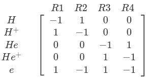
In the Reaction base class, the constructor instantiates a ReactionParser, which assembles one
column of this matrix from the reaction string.
Note
The reaction string is extracted from the comma-separated list of strings provided as the ‘type’
of the reactions component in the input file. All reaction classes (including those that do not
currently inherit from Reaction) inherit from ReactionBase, which ensures that subclasses are
paired up with reaction strings correctly. It is anticipated that changes to the input file
format and/or the migration of all reaction classes to the new framework will make
ReactionBase unnecessary in the future.
Tip
In addition to computing population changes, ReactionParser can be used to identify different
subsets of species via the species_filter enum. For instance, to obtain the names of all
‘heavy’ (non-electron) reactants:
auto heavy_reactants = this->parser.get_species(species_filter::reactants, species_filter::heavy);
Source term equations#
Source terms related to the population changes are calculated from the stoichiometric coefficients
in Reaction::transform_impl.
The reaction rate is calculated as
where \(\langle\sigma_v\rangle\) is the reaction cross section and \(M\) is called the mass action factor.
The density source for a species \(s\) follows directly from the rate:
where \(C_s\) is the population change for species \(s\) (from the stoichiometry matrix) and \(K\) is the reaction rate calculated above. The momentum source (\(F\)) and energy source (\(E\)) associated with a species population change depend on whether the reaction in question is a net consumer (\(C_s < 0\)) or a net producer (\(C_s > 0\)) of the species:
If the species is consumed, it has negative sources proportional to its current momentum (\({NV}_s\)) and energy (\(\mathcal{E}_s\)). If the species is produced, it has positive sources, which are proportional to the total momentum and energy of all consumed reactants (\(r'\); implying \(C_r < 0\)).
\(f_{NV,s}\) and \(f_{\mathcal{E},s}\) are weights / splitting factors used to distribute momentum and energy between products. The default is to weight by mass for momentum, and by population change (number) for energy, that is
where \(m\) are species masses, \(C\) are population changes and subscripts \(s\) and \(p'\) refer to the target species and to a produced species (\(C > 0\)) respectively. \(\Delta M\) and \(\Delta N\) are the change in mass and particle number associated with one instance of the reaction.
These default factors can be overridden by calling
set_energy_channel_weight and
set_momentum_channel_weight in the constructor of a
reaction subclass.
For example, for charge exchange, momentum and energy need to be transferred
from a reactant that donates an electron (‘r1’) to the resulting product (‘p1’) and
from a reactant that accepts an electron (‘r2’) to the resulting product (‘p2’).
The following code sets channels to enforce those requirements:
// Energy exchange between r1 and p1
set_energy_channel_weight(this->r1, this->p1, 1.0);
set_energy_channel_weight(this->r1, this->p2, 0.0);

// Energy exchange between r2 and p2
set_energy_channel_weight(this->r2, this->p1, 0.0);
set_energy_channel_weight(this->r2, this->p2, 1.0);

//  Momentum exchange between r1 and p1
set_momentum_channel_weight(this->r1, this->p1, 1.0);
set_momentum_channel_weight(this->r1, this->p2, 0.0);

// Momentum exchange between r2 and p2
// (Can be turned off for neutral-ion CX using config option)
if (this->has_neutral_reactant && this->no_neutral_cx_mom_gain) {
   set_momentum_channel_weight(this->r2, this->p2, 0.0);
} else {
   set_momentum_channel_weight(this->r2, this->p2, 1.0);
}
set_momentum_channel_weight(this->r2, this->p1, 0.0);
Note
So-called participation factors are included in all source term
calculations in the code. For now, these are all set to 1, reproducing the equations above
exactly, but in future they could be made configurable to allow users to experiment with tuning
the contribution of particular species to reaction source terms.
Source term calculation#
Density, momentum and energy source fields are constructed in Reaction::transform_impl using the
RateHelper class to calculate reaction rates and collision frequencies.
On instantiation, RateHelper assembles maps containing (pointers to) all reactant densities
and any other fields required as inputs.
RateHelper::calc_rates is “run-time templated”, allowing it to accept rate functions with 1D and
2D parameterisations. It also includes an optional flag which causes reaction input parameters to be
averaged in the parallel direction. Averaging is turned on by default, but can be disabled in a
subclass by setting do_parallel_averaging = false.
Having calculated the reaction rate, Reaction::transform_impl constructs sources by looping
over the species population changes provided by ReactionParser.
Note
The loop to compute momentum and energy sources includes a subtle workaround for reactions like
symmetric charge exchange. Rather than using the regular stoichiometric coefficients, which are
all zero in such cases, the loop uses the result of ReactionParser::get_mom_energy_pop_changes().
For symmetric reactions, this returns a std::multimap in which each species appears
twice; once as a reactant, with a negative population change and once as a product, with a
positive population change. This effectively turns reactions like \(\textrm{a} + \textrm{b}
\rightarrow \textrm{b} + \textrm{a}\) into \(\textrm{a} + \textrm{b} \rightarrow \textrm{b}'
+ \textrm{a}'\), allowing the momentum and energy transfer to be computed as usual, before mapping
sources back to the correct species.
Adding new reaction subclasses#
New reaction subclasses should inherit directly or indirectly from Reaction. They are registered
in the code with the reaction string as an argument, e.g.
struct MyReaction : public Reaction {
   ...
}

RegisterComponent<MyReaction> register_myreaction("a + b -> c + d");
Any sources associated with the reaction that are not captured by
transform_impl should be added by overriding
transform_additional and using
update_source to set source terms and associated diagnostics.
Adding new reaction diagnostics#
New diagnostics are configured by making calls to add_diagnostic in the
subclass constructor; e.g. for a density source associated with the neutral reactant in charge
exchange:
r1 is the name of a reactant that
charge-exchanges with reactant r2 creating product p1.#add_diagnostic(
this->r1, fmt::format("S{:s}{:s}_cx", this->r1, this->r2),
fmt::format("Particle transfer to {:s} from {:s} due to CX with {:s}", this->r1,
this->p1, this->r2),
ReactionDiagnosticType::density_src, standard_name, identity,
"particle transfer");
An optional function pointer can be used to set a transformation that will be applied when the
diagnostic is updated. The value passed here (also the default) is identity, meaning that
the diagnostic and associated source term will be updated in the same way. The fourth argument is an
enum value that determines, among other things, which metadata will be set when the
diagnostic is written out.
Each call adds an instance of ReactionDiagnostic to a diagnostics map,
indexed by species name and a ReactionDiagnosticType
enum. The map entries are updated via update_source(), which wraps the
add(), subtract(), and set() operations, applying them to both a source term and to an associated
diagnostic at the same time.
For example, this code
update_source<add<Field3D>>(state, "h+", ReactionDiagnosticType::momentum_src, momentum_source);
would add the momentum_source field to state["species"]["h+"]["momentum_source"],
then apply the diagnostic transform (which defaults to an identity function) to
momentum_source and add the result to any diagnostics of type momentum_src
associated with species h+.
Note
add(), subtract(), and set() can still be used directly to update the state, as usual, if there
is no associated diagnostic to update.
Finally, diagnostics are written out in outputVars(), which simply iterates
over the diagnostics map, copying fields into the output state. Appropriate
metadata is set for each diagnostic depending on the associated ReactionDiagnosticType.
Adding new reaction data#
If the data being added is of a new type (i.e. one not handled by an existing subclass of
ReactionData), developers will need to:
Create a new class that inherits from
ReactionData(or fromReactionDataWithCoeffsif the rate calculation computes a fit value from coefficients).Implement all pure virtual functions, including those that calculate rates with different parameterisations.
Add code to the constructor of the new subclass to read data into the
coeffsdata member, for file-based data sources.Add a new value to the
ReactionDataTypeenum.Register the data class in a new header file.
RegisterReactionData<MyDataClass> register_myclass("mylabel");
where “mylabel” must match the value of the
ReactionDataTypeenum added in step 4, converted to lowercase.Add an include statement for your class’s header in
hermes-3.hxx.
For both new and existing data types, developers need to
Add any associated json data files to the
./json_databasedirectory.Register a
Reactionsubclass for the reaction string.Add any default data IDs to the
generate_default_data_ids_map()function inreaction_settings.hxx.
Step 3. is optional, but without it, users will always need to specify the data type and ID/label for the new reaction in their input file.
Example: To add He+ ionisation: he+ + e -> he+2 + 2e one could
Create
./json_database/AMJUEL_H.4_2.2C.jsoncontaining the relevant coefficients, matching the format of existing Amjuel json files.Register the reaction with the standard ionisation reaction class:
RegisterComponent<IznReaction> register_izn_he2p("he+ + e -> he+2 + 2e");Set the new data to be the default source for He+ ionisation in
include/reaction_settings.hxxstatic inline void generate_default_data_ids_map() { ... add_default_id(ReactionDataTypes::Amjuel, "he+ + e -> he+2 + 2e", ReactionCoeffTypes::sigma_v, "H.4_2.2C"); ... }
Note
For ionisation/recombination one would also need to add data to compute the losses associated with the ionisation potential energy cost and photon emission. At time of writing, appropriate Amjuel data is not available for this reaction, which is why He+ ionisation hasn’t already been added.
Tests#
The specification of the Toro tests used here is taken from Walker (2012), originally from Toro’s book Riemann Solvers and Numerical Methods for Fluid Dynamics.
1D-recycling-dthe#
This is a comprehensive 1D test featuring three species (deuterium tritium and helium) as well as all of the parallel closure terms apart from electron viscosity. It includes ionisation and recombination reactions for all species as well as charge exchange for D-D, T-T, D-T and T-D species pairs.
The test checks the values of charge exchange channels in the final domain cell against a reference.
The test file can be used to generate the test data if gen_data is set to True in the beginning
of the script.
2D-production#
This is a test representing the most common production fidelity simulations at the time of implementation. It features a double null 2D tokamak from an upcoming publication with deuterium only, a neutral puff, H-mode profiles of anomalous diffusion coefficients, a neutral pump, fast/thermal recycling, fast/thermal reflection as well as decay length boundary conditions on the SOL and PFR. Viscosity, impurities, currents and drifts are neglected.
The test downloads the restart files and the grid from Zenodo and runs a few very short timesteps. It compares electron pressure and ion momentum at the four targets, outer midplane, SOL boundary and core/pfr boundaries. If the test fails, it will print the degree of error at each boundary.
The test file can be used to generate the test data if gen_data is set to True in the beginning
of the script.
2D-recycling#
This test uses the same restart file as 2D-production, but tests target recycling by reproducing the relevant recycling.cxx section in Python. It compares the source of recycled neutral density and energy as well as the pumped neutral density and energy sources between the calculation and the reference simulation. The test currently only covers the target and does not reproduce radial recycling or pumping. Because of this, the test neglects the outermost radial domain cells, which can simultaneously have sources due to parallel and radial recycling or pumping.
This test is a reproduction of C++ code, and therefore there is no golden answer reference to update.
This test plots results and can be used to help with developing the recycling component. There
is a plot flag near the beginning of the file.
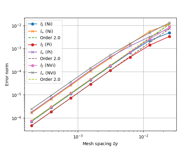
1D fluid (MMS)#
tests/integrated/1D-fluid
This convergence test using the Method of Manufactured Solutions (MMS) solves fluid equations in the pressure form:
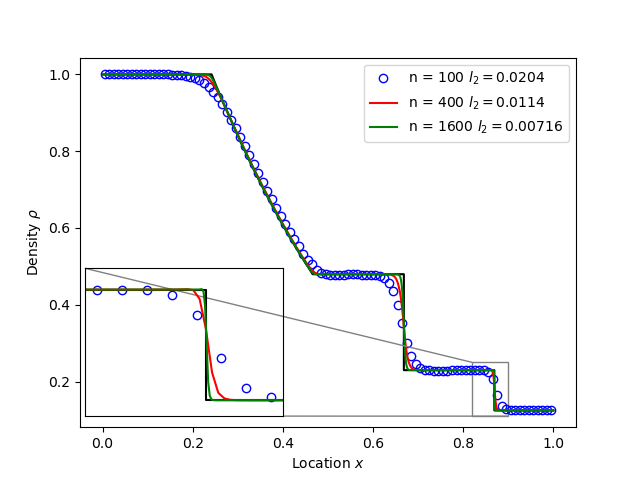
Sod shock#
tests/integrated/sod-shock and tests/integrated/sod-shock-energy
Euler equations in 1D. Starting from a state with a jump at the middle of the domain. Left state density, velocity and pressure are \(\left(\rho_L, u_L, p_L\right) = \left(1.0, 0, 1.0\right)\) Right state \(\left(\rho_R, u_R, p_R\right) = \left(0.125, 0, 0.1\right)\). The result is shown in figure below at time \(t = 0.2\) for different resolutions in a domain of length 1. The solid black line is the analytic solution.
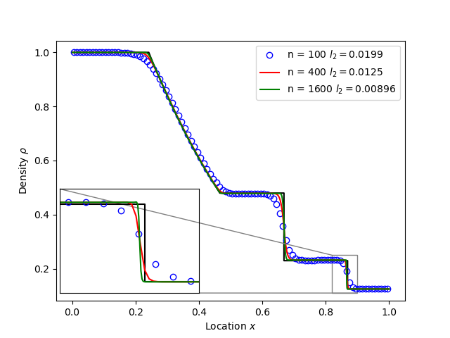
When evolving pressure the position of the shock front lags the analytic solution, with the pressure behind the front slightly too high. This is a known consequence of solving the Euler equations in non-conservative form. If instead we evolve energy (internal + kinetic) then the result is much closer to the analytic solution.
Toro test 1#
tests/integrated/toro-1
Toro’s test problem #1, from Riemann Solvers and Numerical Methods for Fluid Dynamics is a variation of Sod’s shock tube problem. The left state is moving into the right, increasing the speed of the resulting shock. Left state \(\left(\rho_L, u_L, p_L\right) = \left(1.0, 0.75, 1.0\right)\) Right state \(\left(\rho_R, u_R, p_R\right) = \left(0.125, 0, 0.1\right)\). The size of the domain is 5, and the reference result is given at time \(t = 0.8\).
Toro test 2#
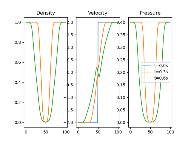
tests/integrated/toro-2 and tests/integrated/toro-2-energy
Toro’s test problem #2 tests robustness to diverging flows and near-zero densities. The initial state has constant density and temperature, but a jump in velocity. Left state \(\left(\rho_L, u_L, p_L\right) = \left(1.0, -2.0, 0.4\right)\) Right state \(\left(\rho_R, u_R, p_R\right) = \left(1.0, 2.0, 0.4\right)\). The result in a domain of length 5 at time \(t=0.6\) is shown below.
Toro test 3#
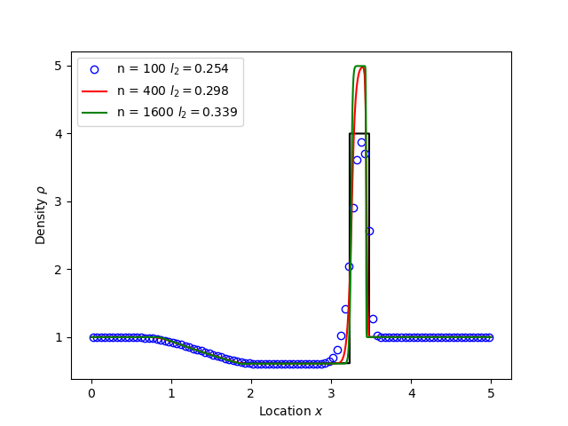
tests/integrated/toro-3 and tests/integrated/toro-3-energy
Toro’s test problem #3 contains a strong shock close to a contact discontinuity. Left initial state \(\left(\rho_L, u_L, p_L\right) = \left(1.0, 0, 1000.0\right)\) Right state \(\left(\rho_R, u_R, p_R\right) = \left(1.0, 0, 0.01\right)\). Time \(t = 0.04\).
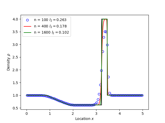
When evolving pressure, the simulation is robust but the density peak does not converge to the analytic solution (solid black line):
However by evolving energy the result converges towards the analytic solution:
Toro test 4#
tests/integrated/toro-4 and tests/integrated/toro-4-energy
Toro’s test problem #4 produces two right-going shocks with a contact between them. Left state \(\left(\rho_L, u_L, p_L\right) = \left(5.99924, 19.5975, 460.894\right)\) Right state \(\left(\rho_R, u_R, p_R\right) = \left(5.99242, -6.19633, 46.0950\right)\). Result at time \(t = 0.15\).
Toro test 5#
tests/integrated/toro-5 and tests/integrated/toro-5-energy
The initial conditions for Toro’s test problem #5 are the same as test #3, but the whole system is moving to the left at a uniform speed. The velocity is chosen so that the contact discontinuity remains almost stationary at the initial jump location. Left state \(\left(\rho_L, u_L, p_L\right) = \left(1, -19.59745, 1000.0\right)\) Right state \(\left(\rho_R, u_R, p_R\right) = \left(1, -19.59745, 0.01\right)\). Result at time \(t = 0.03\).
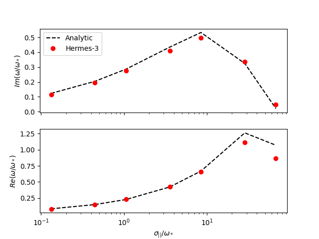
Drift wave#
tests/integrated/drift-wave
This calculates the growth rate and frequency of a resistive drift wave with finite electron mass.
The equations solved are:
Linearising around a stationary background with constant density \(n_0\) and temperature \(T_0\), using \(\frac{\partial}{\partial t}\rightarrow -i\omega\) gives:
where the radial density length scale coming from the radial \(E\times B\) advection of density is defined as
Substituting and rearranging gives:
or
where
This is a cubic dispersion relation, so we find the three roots (using NumPy), and choose the root with the most positive growth rate (imaginary component of \(\omega\)).
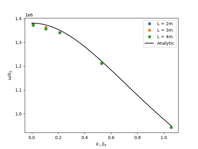
Alfven wave#
The equations solved are
Linearising around a stationary background with constant density \(n_0\) and temperature \(T_0\), using \(\frac{\partial}{\partial t}\rightarrow -i\omega\) gives:
Rearranging results in a quadratic dispersion relation:
where \(V_A = B / \sqrt{\mu_0 n_0 m_i}\) is the Alfven speed, and \(c / \omega_{pe} = \sqrt{m_e / \left(\mu_0 n_0 e^2\right)}\) is the electron skin depth.
When collisions are neglected, we obtain the result
Collision frequency selection#
There are two simple integrated tests to make sure that the collision frequency selection is correct
across neutral_mixed, evolve_pressure, ion_viscosity and neutral_parallel_diffusion.
A minimal 3D geometry is run for one RHS evaluation, and the test checks the log file
to make sure the correct collisionalities were selected. One of the tests is for the multispecies
mode across all components, while the other is for braginskii for plasma and afn for neutrals.