Examples#
Hermes-3 contains a large number of example simulations, with only a selection
shown here. Please refer to the examples directory for more.
As the development of the code has progressed rapidly, it has been difficult to keep all of the examples up to date and not all are guaranteed to represent the most optimal setup.
A review is currently in process to select a few of the most useful examples and keep them up to date regularly, with the remaining examples being updated in the future.
So far, only 1D example cases received this treatment, resulting in a new,
updated example 1D-threshold and the remaining 1D cases moved to examples/1D-tokamak/extra.
Note that many will likely work with no modifications.
1D Field line#
In 1D, Hermes-3 follows a single flux tube, typically from midplane to target. The code inherits a lot of capability and convention from the code SD1D - see Dudson 2019. for a good description of the equations and capabilities. Note that SD1D features a “plasma” pressure equation, combining the ion and electron pressures, which are separate in Hermes-3.
There is an xHermes 1D post-processing example to guide you through results analysis.
For published Hermes-1D applications, see Body 2024 and Holt 2024.
1D-threshold#
This simulates a similar setup to the SD1D code: A 1D domain, with a source of heat and particles on one side, and a sheath boundary on the other. Ions recycle into neutrals, which charge exchange and are ionised. A difference is that separate ion and electron temperatures are evolved here.
Fig. 3 Evolution of ion and neutral density (blue); ion, electron and neutral temperature (red), starting from flat profiles.#
Due to the short length-scales near the sheath, the grid is packed close to the target, by setting the grid spacing to be a linear function of index:
[mesh]
dy = (length / ny) * (1 + (1-dymin)*(1-y/pi))
where dymin is 0.1 here, and sets the smallest grid spacing (at the
target) as a fraction of the average grid spacing.
The components are ion species d+, atoms d, electrons e:
[hermes]
components = (d+, d, e,
              sheath_boundary_simple, braginskii_collisions,
              braginskii_friction, braginskii_heat_exchange,
              recycling, reactions, electron_force_balance,
              neutral_parallel_diffusion, braginskii_conduction)
The electron velocity is set to the ion by specifying zero_current; A sheath boundary is included; Collisions are needed to be able to calculate heat conduction, as well as neutral diffusion rates; Recycling at the targets provides a source of atoms; 1D: neutral_parallel_diffusion simulates cross-field diffusion in a 1D system. The electron force balance links electron pressure gradient with the ion momentum equation. Please see the relevant documentation pages about these components for further information.
The sheath boundary is only imposed on the upper Y boundary:
[sheath_boundary_simple]

lower_y = false
upper_y = true
The reactions component is a group, which lists the reactions included:
[reactions]
type = (
        d + e -> d+ + 2e,   # Deuterium ionisation
        d+ + e -> d,          # Deuterium recombination
        d + d+ -> d+ + d,   # Charge exchange
       )
2D Drift-plane#
Simulations where the dynamics along the magnetic field is not included, or only included in a parameterised way as sources or sinks. The field line direction is then “into the page”, and the domain represents a slice somewhere along the field line, e.g. at the midplane. These are useful for the study of the basic physics of plasma “blobs” / filaments, and tokamak edge turbulence.
Blob2d#
A seeded plasma filament in 2D. This version is isothermal and cold ion, so only the electron density and vorticity are evolved. A sheath-connected closure is used for the parallel current.
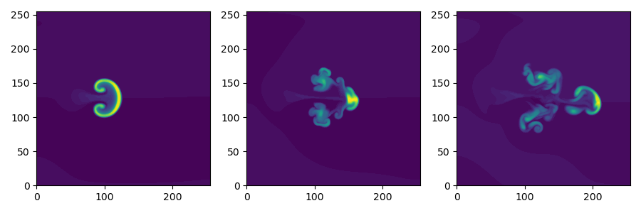
Fig. 4 Electron density Ne at three times, showing propagation to the right#
The model components are
[hermes]
components = e, vorticity, sheath_closure
The electron component consists of two types:
[e]  # Electrons
type = evolve_density, isothermal
The evolve_density component type evolves the electron density Ne. This component
has several options, which are set in the same section e.g.
poloidal_flows = false # Y flows due to ExB
and so solves the equation:
The isothermal component type sets the temperature to be a constant, and using
the density then sets the pressure. The constant temperature is also
set in this [e] section:
temperature = 5 # Temperature in eV
so that the equation solved is
where \(T_e\) is the fixed electron temperature (5eV).
The vorticity component uses the pressure to calculate the diamagnetic current,
so must come after the e component. This component then calculates the potential.
Options to control the vorticity component are set in the [vorticity] section.
The sheath_closure component uses the potential, so must come after vorticity.
Options are also set as
[sheath_closure]
connection_length = 10 # meters
This adds the equation
where \(L_{||}\) is the connection length.
Blob2D-Te-Ti#
A seeded plasma filament in 2D. This version evolves both electron and ion temperatures. A sheath-connected closure is used for the parallel current.
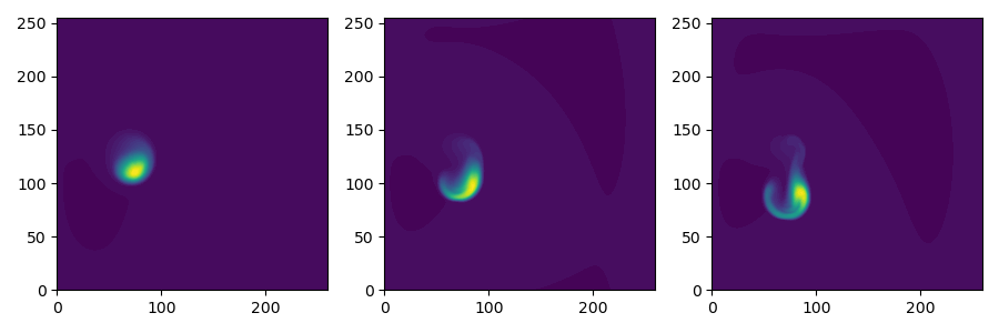
Fig. 5 Electron density Ne at three times, showing propagation to the right and downwards#
The model components are
[hermes]
components = e, h+, vorticity, sheath_closure
The electron component evolves density (saved as Ne) and pressure
(Pe), and from these the temperature is calculated.
[e]
type = evolve_density, evolve_pressure
The ion component sets the ion density from the electron density, by
using the quasineutrality of the plasma; the ion pressure (Ph+) is evolved.
[h+]
type = quasineutral, evolve_pressure
The equations this solves are similar to the previous Blob2d case, except now there are pressure equations for both ions and electrons:
2D-drift-plane-turbulence-te-ti#
A 2D turbulence simulation, similar to the Blob2D-Te-Ti case, but with extra source and sink terms, so that a statistical steady state of source-driven turbulence can be reached.
The model components are
[hermes]
components = e, h+, vorticity, sheath_closure
The electron component evolves density (saved as Ne) and pressure
(Pe), and from these the temperature is calculated.
[e]
type = evolve_density, evolve_pressure
The ion component sets the ion density from the electron density, by
using the quasineutrality of the plasma; the ion pressure (Ph+) is evolved.
[h+]
type = quasineutral, evolve_pressure
The sheath closure now specifies that additional sink terms should be added
[sheath_closure]
connection_length = 50 # meters
potential_offset = 0.0  # Potential at which sheath current is zero
sinks = true
and radially localised sources are added in the [Ne], [Pe], and [Ph+]
sections.
The equations this solves are the same as the previous Blob2D-Te-Ti case, except wih extra source and sink terms. In SI units (except temperatures in eV) the equations are:
Where \(\overline{T}\) and \(\overline{n}\) are the reference temperature (units of eV) and density (in units of \(m^{-3}\)) used for normalisation. \(\overline{c_s} = \sqrt{e\overline{T} / m_p}\) is the reference sound speed, where \(m_p\) is the proton mass. The mean ion atomic mass \(\overline{A}\) is set to 1 here.
These reference values enter into the sheath current \(\mathbf{j}_{sh}\) because that is a simplified, linearised form of the full expression. Likewise the vorticity (\(\omega\)) equation used the Boussinesq approximation to simplify the polarisation current term, leading to constant reference values being used.
The sheath heat transmission coefficients default to \(\gamma_e = 6.5\) and \(\gamma_i = 2.0\) (\(\gamma_i\) as suggested in Stangeby’s textbook between equations (2.92) and (2.93)). Note the sinks in may not be correct or the best choices, especially for cases with multiple ion species; they were chosen as being simple to implement by John Omotani in May 2022.
2D Axisymmetric SOL#
These are transport simulations, where the cross-field transport is given by diffusion, and fluid-like equations are used for the parallel dynamics (as in the 1D flux tube cases).
The input settings (in BOUT.inp) are set to read the grid from a file tokamak.nc.
This is linked to a default file compass-36x48.grd.nc, a COMPASS-like lower single
null tokamak equilibrium. Due to the way that BOUT++ uses communications between
processors to implement branch cuts, these simulations require a multiple of 6 processors.
You don’t usually need 6 physical cores to run these cases, if MPI over-subscription
is enabled.
heat-transport#
In examples/tokamak/heat-transport, this evolves only electron pressure with
a fixed density. It combines cross-field diffusion with parallel heat conduction
and a sheath boundary condition.
To run this simulation with the default inputs requires (at least) 6 processors because it is a single-null tokamak grid. From the build directory:
cd examples/tokamak
mpirun -np 6 ../../hermes-3 -d heat-transport
That will read the grid from tokamak.nc, which by default links to
the compass-36x48.grd.nc file.
The components of the model are given in heat-transport/BOUT.inp:
[hermes]
components = (e, h+,
              braginskii_collisions, braginskii_friction, braginskii_heat_exchange,
              sheath_boundary_simple, braginskii_conduction)
We have two species, electrons and hydrogen ions, and add collisions between them and a simple sheath boundary condition.
The electrons have the following components to fix the density, evolve the pressure, and include anomalous cross-field diffusion:
[e]
type = fixed_density, evolve_pressure, anomalous_diffusion
The fixed_density takes these options:
AA = 1/1836
charge = -1
density = 1e18 # Fixed density [m^-3]
so in this simulation the electron density is a uniform and constant value.
If desired, that density can be made a function of space (x and y coordinates).
The evolve_pressure component has thermal conduction enabled, and outputs
extra diagnostics i.e. the temperature Te:
thermal_conduction = true   # Spitzer parallel heat conduction
diagnose = true   # Output additional diagnostics
There are other options that can be set to modify the behavior,
such as setting kappa_limit_alpha to a value between 0 and 1 to impose
a free-streaming heat flux limit.
Since we’re evolving the electron pressure we should set initial and
boundary conditions on Pe:
[Pe]
function = 1
bndry_core = dirichlet(1.0)  # Core boundary high pressure
bndry_all = neumann
That sets the pressure initially uniform, to a normalised value of 1,
and fixes the pressure at the core boundary. Other boundaries are set
to zero-gradient (neumann) so there is no cross-field diffusion of heat out of
the outer (SOL or PF) boundaries. Flow of heat through the sheath is
governed by the sheath_boundary_simple top-level component.
The hydrogen ions need a density and temperature in order to calculate the collision frequencies. If the ion temperature is fixed to be the same as the electron temperature then there is no transfer of energy between ions and electrons:
[h+]
type = quasineutral, set_temperature
The quasineutral component sets the ion density so that there is no net charge
in each cell. In this case that means the hydrogen ion density is set equal to
the electron density. To perform this calculation the component requires that the
ion atomic mass and charge are specified:
AA = 1
charge = 1
The set_temperature component sets the ion temperature to the temperature of another
species. The name of that species is given by the temperature_from option:
temperature_from = e # Set Th+ = Te
The braginskii_collisions component is described in the manual, and
calculates both electron-electron and electron-ion collisions. These
can be disabled if desired, using individual options. There are also
ion-ion, electron-neutral, ion-neutral and neutral-neutral collisions
that are not used here.
The sheath_boundary_simple component is a simplified Bohm-Chodura sheath boundary
condition, that allows the sheath heat transmission coefficient to be specified for
electrons and (where relevant) for ions.
The equations solved by this example are:
The calculation of the Coulomb logarithms follows the NRL formulary,
and the above expression is used for temperatures above 10eV. See the
braginskii_collisions manual section for the expressions used in
other regimes.
recycling-dthene#
- Warning
Impurity transport can be notoriously computationally expensive to run. If you are interested in 2D transport simulations, consider starting with the much simpler
recyclingexample (not yet in documentation)
The recycling-dthene example includes cross-field diffusion,
parallel flow and heat conduction, collisions between species, sheath
boundary conditions and recycling. It simulates the density, parallel
flow and pressure of the electrons; ion species D+, T+, He+, Ne+; and
neutral species D, T, He, Ne.
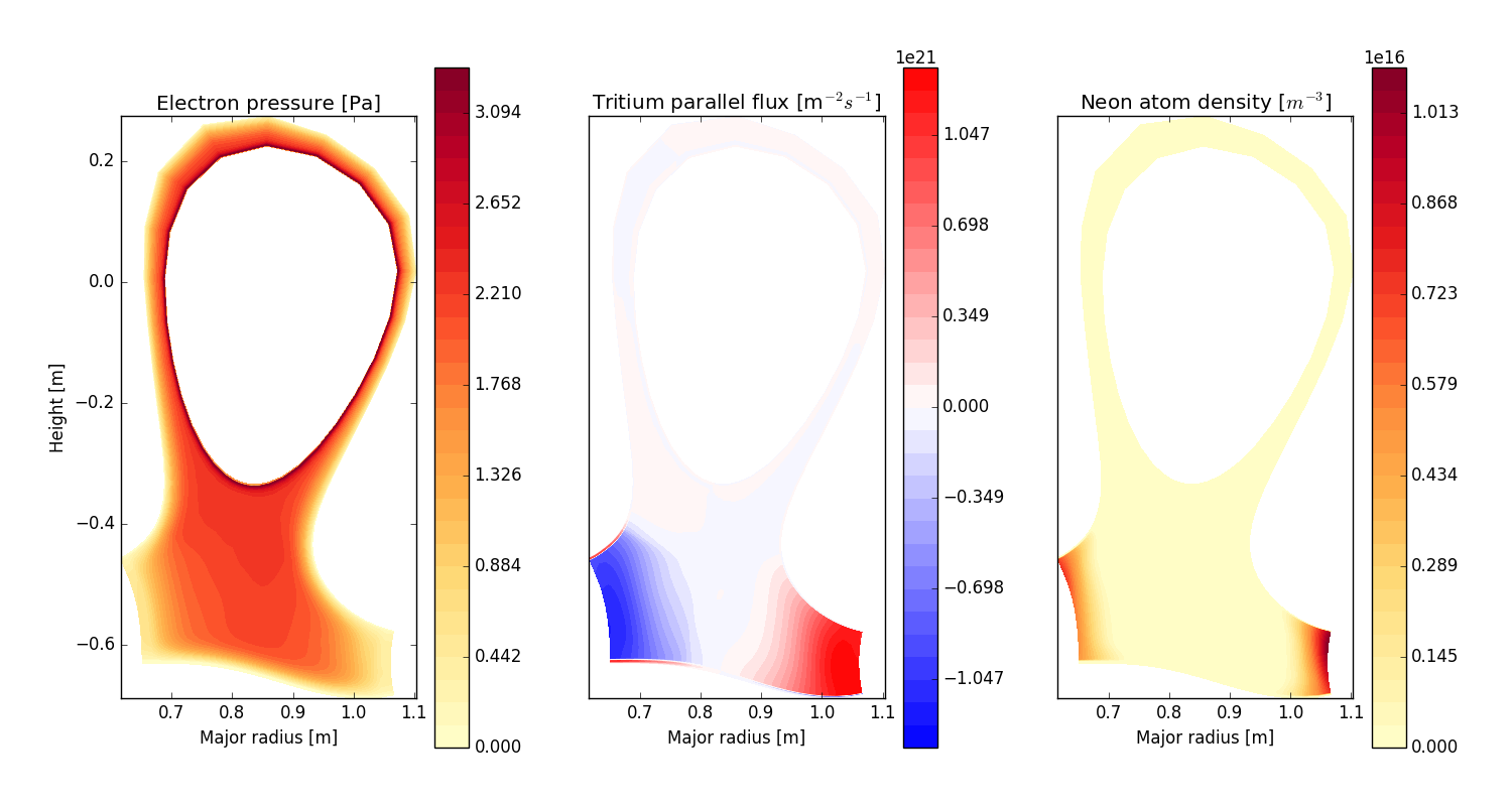
Fig. 6 Electron pressure, parallel tritium flux, and neon atom density. Simulation evolves D, T, He, Ne and electron species, including ions and neutral atoms.#
The model components are a list of species, and then collective components which couple multiple species.
[hermes]
components = (d+, d, t+, t, he+, he, ne+, ne, e, braginskii_collisions,
              braginskii_friction, braginskii_heat_exchange, sheath_boundary,
              recycling, reactions, braginskii_conduction)
Note that long lists like this can be split across multiple lines by using parentheses.
Each ion species has a set of components, to evolve the density, momentum and pressure. Anomalous diffusion adds diffusion of particles, momentum and energy. For example deuterium ions contain:
[d+]
type = evolve_density, evolve_momentum, evolve_pressure, anomalous_diffusion
AA = 2
charge = 1
Atomic reactions are specified as a list:
[reactions]
type = (
     d + e -> d+ + 2e,   # Deuterium ionisation
     t + e -> t+ + 2e,   # Tritium ionisation
     he + e -> he+ + 2e, # Helium ionisation
     he+ + e -> he,      # Helium+ recombination
     ne + e -> ne+ + 2e, # Neon ionisation
     ne+ + e -> ne,      # Neon+ recombination
    )
3D Turbulence#
turbulence#
In this example, Hermes-3 is configured to solve an electrostatic 6-field model for vorticity, electron density, electron and ion parallel velocity, electron and ion pressure.
The input file is in the Hermes-3 repository under
examples/tokamak-2D/turbulence.
The lines that define the components to include in the model are:
[hermes]
components = (e, d+, sound_speed, vorticity,
              sheath_boundary, braginskii_collisions, braginskii_friction,
              braginskii_heat_exchange, diamagnetic_drift, classical_diffusion,
              polarisation_drift, braginskii_conduction
             )

[e]
type = evolve_density, evolve_pressure, evolve_momentum

[d+]
type = quasineutral, evolve_pressure, evolve_momentum
We define two species: electrons e and deuterium ions d+.
Electron density is evolved, and ion density is set to electron
density by quasineutrality. The electron fluid equations for density
\(n_e\), parallel momentum \(m_en_ev_{||e}\), and pressure
\(p_e = en_eT_e\) are:
Here the electrostatic approximation is made, so \(E_{||} = -\mathbf{b}\cdot\nabla\phi\).
The ion fluid equations assume quasineutrality so \(n_i = n_e\), and evolve the ion parallel momentum \(m_in_iv_{||i}\) and pressure \(p_i\):
The vorticity \(\omega\) is
whose evolution is given by the current continuity equation:
where the Boussinesq approximation is made, replacing the density in the polarisation current with a constant \(\overline{n}\). The divergence of the diamagnetic current is written as
The input file sets the number of output steps to take and the time between outputs in units of reference ion cyclotron time:
nout = 10      # Number of output steps
timestep = 10  # Output timestep, normalised ion cyclotron times [1/Omega_ci]
With the normalisations in the input that reference time is about 1e-8 seconds, so taking 10 steps of 10 reference cyclotron times each advances the simulation by around 1 microsecond in total.
The first few steps are likely to be slow, but the simulation should speed up considerably by the end of these 10 steps. This is largely due to rapid transients as the electric field is set up by the sheath and parallel electron flows.
Note: When starting a new simulation, it is important to calibrate the input sources, to ensure that the particle and power fluxes are what you intend.
The inputs are electron density source, electron and ion heating power.
The particle source is set in the electron density section [Ne]:
[Ne]
flux = 3e21 # /s
shape_factor = 1.0061015504152746

source = flux * shape_factor * exp(-((x - 0.05)/0.05)^2)
source_only_in_core = true
The inputs read by Hermes-3/BOUT++ are source and
source_only_in_core. The flux and shape_factor values are
just convenient ways to calculate the source (New variables can be
defined and used, and their order in the input file doesn’t matter).
A turbulence simulation typically takes many days of running, to reach (quasi-)steady state then gather statistics for analysis. To continue a simulation, the simulation state is loaded from restart files (BOUT.restart.*) and the simulation continues running. The “nout” and “timestep” set the number of new steps to take. To do this, copy the BOUT.inp (options) file and BOUT.restart.* files into a new directory. For example, if the first simulation was in a directory “01”:
$ mkdir 02
$ cp 01/BOUT.inp 02/
$ cp 01/BOUT.restart.* 02/
We now have a new input file (02/BOUT.inp) that we can edit to update
settings. I recommend increasing the output timestep from 10 to 100,
and the number of outputs nout from 10 to 100. You can also adjust
particle and power sources, or make other changes to the settings. Once
ready, restart the simulation:
$ mpirun -np 64 ./hermes-3 -d 02 restart
Note the restart argument.
TCV-X21#
An example based on the TCV validation in Oliveira, Body et al. 2022,
located in located in examples\tcv-x21.