Tests

The specification of the Toro tests used here is taken from Walker (2012), originally from Toro’s book Riemann Solvers and Numerical Methods for Fluid Dynamics.

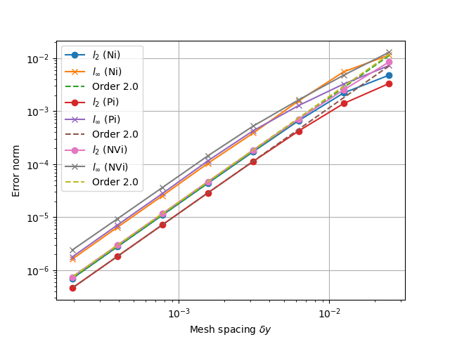
1D fluid (MMS)

tests/integrated/1D-fluid

This convergence test using the Method of Manufactured Solutions (MMS) solves fluid equations in the pressure form:

\[\begin{split}\begin{aligned} \frac{\partial n}{\partial t} &= -\nabla\cdot\left(n\mathbf{b}v_{||}\right) \\ \frac{\partial p}{\partial t} &= -\nabla\cdot\left(p\mathbf{b}v_{||}\right) - \frac{2}{3}p\nabla\cdot\left(\mathbf{b}v_{||}\right) \\ \frac{\partial}{\partial t}\left(mnv_{||}\right) &= -\nabla\cdot\left(nv_{||}\mathbf{b}v_{||}\right) - \partial_{||}p \end{aligned}\end{split}\]

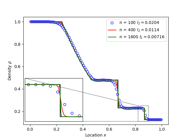
Sod shock

tests/integrated/sod-shock and tests/integrated/sod-shock-energy

Euler equations in 1D. Starting from a state with a jump at the middle of the domain. Left state density, velocity and pressure are \(\left(\rho_L, u_L, p_L\right) = \left(1.0, 0, 1.0\right)\) Right state \(\left(\rho_R, u_R, p_R\right) = \left(0.125, 0, 0.1\right)\). The result is shown in figure below at time \(t = 0.2\) for different resolutions in a domain of length 1. The solid black line is the analytic solution.

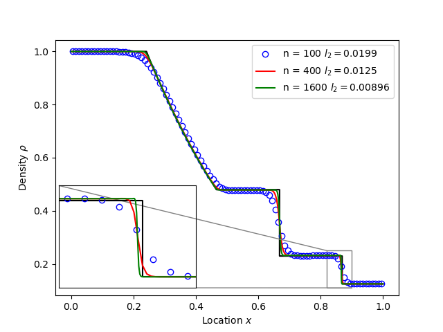
When evolving pressure the position of the shock front lags the analytic solution, with the pressure behind the front slightly too high. This is a known consequence of solving the Euler equations in non-conservative form. If instead we evolve energy (internal + kinetic) then the result is much closer to the analytic solution.

Toro test 1

tests/integrated/toro-1

Toro’s test problem #1, from Riemann Solvers and Numerical Methods for Fluid Dynamics is a variation of Sod’s shock tube problem. The left state is moving into the right, increasing the speed of the resulting shock. Left state \(\left(\rho_L, u_L, p_L\right) = \left(1.0, 0.75, 1.0\right)\) Right state \(\left(\rho_R, u_R, p_R\right) = \left(0.125, 0, 0.1\right)\). The size of the domain is 5, and the reference result is given at time \(t = 0.8\).

Toro test 2

tests/integrated/toro-2 and tests/integrated/toro-2-energy

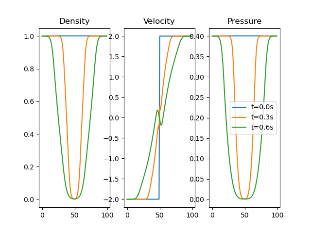
Toro’s test problem #2 tests robustness to diverging flows and near-zero densities. The initial state has constant density and temperature, but a jump in velocity. Left state \(\left(\rho_L, u_L, p_L\right) = \left(1.0, -2.0, 0.4\right)\) Right state \(\left(\rho_R, u_R, p_R\right) = \left(1.0, 2.0, 0.4\right)\). The result in a domain of length 5 at time \(t=0.6\) is shown below.

Toro test 3

tests/integrated/toro-3 and tests/integrated/toro-3-energy

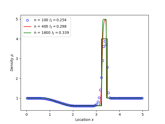
Toro’s test problem #3 contains a strong shock close to a contact discontinuity. Left initial state \(\left(\rho_L, u_L, p_L\right) = \left(1.0, 0, 1000.0\right)\) Right state \(\left(\rho_R, u_R, p_R\right) = \left(1.0, 0, 0.01\right)\). Time \(t = 0.04\).

When evolving pressure, the simulation is robust but the density peak does not converge to the analytic solution (solid black line):

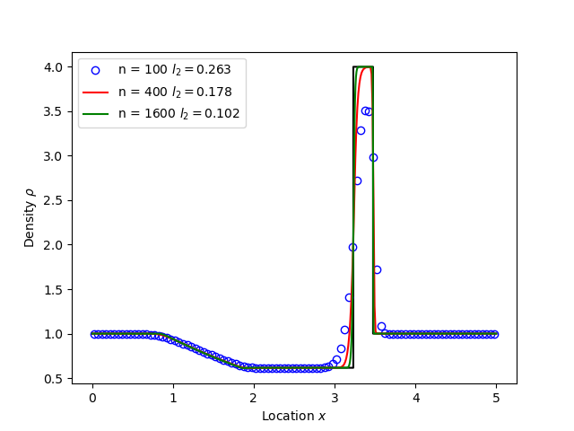
However by evolving energy the result converges towards the analytic solution:

Toro test 4

tests/integrated/toro-4 and tests/integrated/toro-4-energy

Toro’s test problem #4 produces two right-going shocks with a contact between them. Left state \(\left(\rho_L, u_L, p_L\right) = \left(5.99924, 19.5975, 460.894\right)\) Right state \(\left(\rho_R, u_R, p_R\right) = \left(5.99242, -6.19633, 46.0950\right)\). Result at time \(t = 0.15\).

Toro test 5

tests/integrated/toro-5 and tests/integrated/toro-5-energy

The initial conditions for Toro’s test problem #5 are the same as test #3, but the whole system is moving to the left at a uniform speed. The velocity is chosen so that the contact discontinuity remains almost stationary at the initial jump location. Left state \(\left(\rho_L, u_L, p_L\right) = \left(1, -19.59745, 1000.0\right)\) Right state \(\left(\rho_R, u_R, p_R\right) = \left(1, -19.59745, 0.01\right)\). Result at time \(t = 0.03\).

Drift wave

tests/integrated/drift-wave

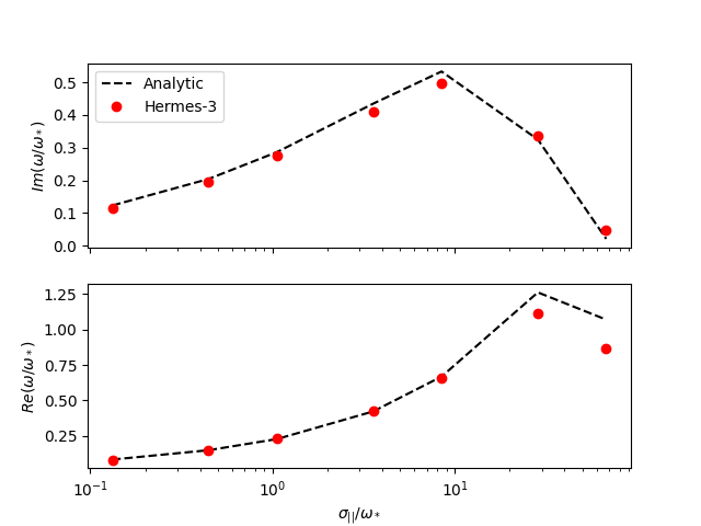
This calculates the growth rate and frequency of a resistive drift wave with finite electron mass.

The equations solved are:

\[\begin{split}\begin{aligned} \frac{\partial n_i}{\partial t} =& -\nabla\cdot\left(n_i\mathbf{v}_{E\times B}\right) \\ n_e =& n_i \\ \frac{\partial}{\partial t}\nabla\cdot\left(\frac{n_0 m_i}{B^2}\nabla_\perp\phi\right) =& \nabla_{||}J_{||} = -\nabla_{||}\left(en_ev_{||e}\right) \\ \frac{\partial}{\partial t}\left(m_en_ev_{||e}\right) =& -\nabla\cdot\left(m_en_ev_{||e} \mathbf{b}v_{||e}\right) + en_e\partial_{||}\phi - \partial_{||}p_e - 0.51\nu_{ei}n_im_ev_{||e} \end{aligned}\end{split}\]

Linearising around a stationary background with constant density \(n_0\) and temperature \(T_0\), using \(\frac{\partial}{\partial t}\rightarrow -i\omega\) gives:

\[\begin{split}\begin{aligned} \tilde{n} =& \frac{k_\perp}{\omega}\frac{n_0}{BL_n}\tilde{\phi} \\ \tilde{\phi} =& -\frac{k_{||}}{\omega k_\perp^2}\frac{eB^2}{m_i}\tilde{v_{||e}} \\ \omega m_e \tilde{v_{||e}} =& -ek_{||}\tilde{\phi} + ek_{||}\frac{T_o}{n_0}\tilde{n} - i0.51\nu_{ei}m_e\tilde{v_{||e}} \end{aligned}\end{split}\]

where the radial density length scale coming from the radial \(E\times B\) advection of density is defined as

\[\frac{1}{L_n} \equiv \frac{1}{n_0}\frac{\partial n_0}{\partial r}\]

Substituting and rearranging gives:

\[i\left(\frac{\omega}{\omega*}\right)^3 \frac{\omega_*}{0.51\nu_{ei}} = \left(\frac{\omega}{\omega_*} - 1\right)\frac{i\sigma_{||}}{\omega_*} + \left(\frac{\omega}{\omega*}\right)^2\]

or

\[\frac{\omega_*}{0.51\nu_{ei}}\left(\frac{\omega}{\omega_*}\right)^3 + i\left(\frac{\omega}{\omega_*}\right)^2 - \frac{\sigma_{||}}{\omega_*}\left(\frac{\omega}{\omega_*}\right) + \frac{\sigma_{||}}{\omega_*} = 0\]

where

\[\begin{split}\begin{aligned} \omega_* =& \frac{k_\perp T_0}{BL_n} \\ \sigma_{||} =& \frac{k_{||}^2}{k_\perp^2}\frac{\Omega_i\Omega_e}{0.51\nu_{ei}} \\ \Omega_s =& eB / m_s \end{aligned}\end{split}\]

This is a cubic dispersion relation, so we find the three roots (using NumPy), and choose the root with the most positive growth rate (imaginary component of \(\omega\)).

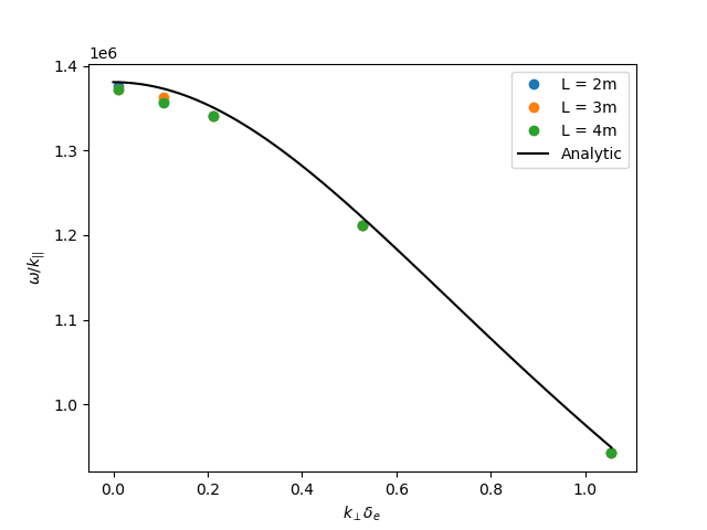
Alfven wave

The equations solved are .. math:

\begin{aligned}
\frac{\partial}{\partial t}\nabla\cdot\left(\frac{n_0 m_i}{B^2}\nabla_\perp\phi\right) =& \nabla_{||}J_{||} = -\nabla_{||}\left(en_ev_{||e}\right) \\
\frac{\partial}{\partial t}\left(m_en_ev_{||e} - en_eA_{||}\right) =& -\nabla\cdot\left(m_en_ev_{||e} \mathbf{b}v_{||e}\right) + en_e\partial_{||}\phi - 0.51\nu_{ei}n_im_ev_{||e} \\
J_{||} =& \frac{1}{\mu_0}\nabla_\perp^2 A_{||}
\end{aligned}

Linearising around a stationary background with constant density \(n_0\) and temperature \(T_0\), using \(\frac{\partial}{\partial t}\rightarrow -i\omega\) gives:

\[\begin{split}\begin{aligned} \tilde{\phi} =& -\frac{k_{||}}{\omega k_\perp^2}\frac{eB^2}{m_i}\tilde{v_{||e}} \\ \omega \left( m_e \tilde{v_{||e}} - e\tilde{A}_{||}\right) =& -ek_{||}\tilde{\phi} - i0.51\nu_{ei}m_e\tilde{v_{||e}} \\ en_0\tilde{v_{||e}} =& -\frac{k_\perp^2}{\mu_0}\tilde{A}_{||} \end{aligned}\end{split}\]

Rearranging results in a quadratic dispersion relation:

\[\omega^2\left(1 + \frac{k_\perp^2 c^2}{\omega_{pe}^2}\right) + i 0.51\nu_{ei}\frac{k_\perp^2 c^2}{\omega_{pe}^2\omega - k_{||}^2V_A^2 = 0\]

where \(V_A = B / \sqrt{\mu_0 n_0 m_i}\) is the Alfven speed, and \(c / \omega_{pe} = \sqrt{m_e / \left(\mu_0 n_0 e^2\right)}\) is the electron skin depth.

When collisions are neglected, we obtain the result

\[\omega^2 = V_A^2\frac{k_{||}^2}{1 + k_\perp^2 c^2 / \omega_{pe}^2}\]